2 Data processing
In this section I’ll process the raw data so that I can use them for analysis in the next section. Note that the data were slightly preprocessed: I only selected variables that we use for processing and analysis here. Other than that, the data were untouched.
The data are on the OSF.
You can download them if you set the code chunk below to eval=TRUE.
Downloading only works when the OSF project is public.
If it isn’t during peer review, you’ll need to paste the data files from the OSF to the data/ folder manually.
# create directory
dir.create("data/", FALSE, TRUE)

# download models
osf_retrieve_node("https://osf.io/yn7sx/?view_only=2d0d8bf4850d4ace8a08c860bc45e9f2") %>%
  osf_ls_nodes() %>%
  filter(name == "data") %>%
  osf_ls_files(
    .,
    n_max = Inf
  ) %>%
  osf_download(
    .,
    path = here("data"),
    progress = FALSE
  )
## # A tibble: 5 x 4
## name id local_path meta
## <chr> <chr> <chr> <list>
## 1 wave1.csv 60746bd2f2ad330543a747fa data/wave1.csv <named list [3]>
## 2 example_id.csv 60746bd2f2ad330543a747ff data/example_id.csv <named list [3]>
## 3 waves_2_to_6.csv 60746bd351f7ae051cf51cc6 data/waves_2_to_6.csv <named list [3]>
## 4 codebook.xlsx 60746be8f6585f051e61be70 data/codebook.xlsx <named list [3]>
## 5 processed_data.rds 60747466f6585f051b61b85e data/processed_data.rds <named list [3]>2.1 Read waves 2-6
We’ll start with loading the data for waves 2 to 6.
We start here instead of wave 1 because participant identification isn’t super straightforward.
A participant doesn’t get a single unique identifier that’s stable across all waves.
Instead, participants start with an ID in wave 1 (called transaction_idOld in the wave 2 to 6 data) and get a new unique ID for wave 2 and so on.
I believe originally the researchers wanted to go with a single ID, but changed their mind.
Look at the data table below (2.1), where I made up two participants to recreate the data structure.
We see that the first participant has an transaction ID (transaction_idOld) for the first wave.
The same participant then has that same old transaction ID for wave two, plus a new transaction ID for wave 2 (transaction_id).
transaction_idW2).
Next to that new variable, is the unique ID for that wave (transaction_idW3).
After that, each new wave has the ID of the previous wave plus a new ID for the current wave.
| id | transaction_old | transaction_id | transaction_idW2 | transaction_idW3 | transaction_idW4 | transaction_idW5 | transaction_idW6 | week |
|---|---|---|---|---|---|---|---|---|
| 1 | 978344791 | NA | NA | NA | NA | NA | NA | 1 |
| 1 | 978344791 | 987910814 | NA | NA | NA | NA | NA | 2 |
| 1 | NA | NA | 987910814 | 994717737 | NA | NA | NA | 3 |
| 1 | NA | NA | NA | 994717737 | 998317051 | NA | NA | 4 |
| 1 | NA | NA | NA | NA | 998317051 | 1005222579 | NA | 5 |
| 1 | NA | NA | NA | NA | NA | 1005222579 | 1018946937 | 6 |
| 2 | 978344792 | NA | NA | NA | NA | NA | NA | 1 |
| 2 | 978344792 | 987910815 | NA | NA | NA | NA | NA | 2 |
| 2 | NA | NA | 987910815 | NA | NA | NA | NA | 3 |
| 2 | NA | NA | NA | NA | NA | NA | NA | 4 |
| 2 | NA | NA | NA | NA | NA | NA | NA | 5 |
| 2 | NA | NA | NA | NA | NA | NA | NA | 6 |
Unfortunately, the id column from the example isn’t included in the raw data, so we’ll have to recreate participant IDs that are constant across waves.
I solved this problem with a loop, which is definitely not the most elegant way to go about this, but I think it gets the job done.
First, lets load the data.
waves_2_to_6 <-
  read_csv(
    here("data", "waves_2_to_6.csv"),
    guess_max = 2e4
  ) %>%
  select(-X1) # remove rownumber
Next, the logic behind assigning the constant IDs. We’ll start at the ID of wave 2, find the ID of wave 3 that’s on the same line as the ID of wave 2 and store the ID for wave 3. We repeat this procedure for all waves and in the end assign an ID to those rows that have the IDs we extracted on any of the ID variables.
The steps, concretely:
- We store all IDs (so that’s the IDs of wave 2) in a vector (excluding
NAs). - Initiate an ID counter (i.e., the participant number we assign later).
- We iterate over each wave 2 ID.
- If participants did participate in a wave, we find the wave 3 ID that is on the same row as the wave 2 that we’re currently looking for.
- We now look for the wave 3 ID and store the wave 4 ID that’s on the same line.
- We repeat that until we’re at the last ID and have all IDs for that participant stored in a vector.
- Then a row gets assigned the participant ID (to the existing, but empty
idvariable) if any of the wave ID variables have a match in the extracted IDs.
On my machine, the below code takes about three minutes.
# the unique wave 2 IDs
ids <- waves_2_to_6 %>%
  pull(transaction_id) %>%
  na.omit

# the participant number we assign later
id_counter <- 1

# assign the correct variable type to the empty ID variable that's already in the data where we'll assign participant numbers at the end of the loop
waves_2_to_6$id <- NA_real_

for (an_id in ids) {

  # transaction ids that belong to that one participant
  id_to_match <- c()

  # add the initial id
  id_to_match <- c(id_to_match, an_id)

  # assign that id as temporary ID for which we should match (id_to_match only has one entry so far)
  temp_id <- id_to_match

  # at this point, participants might have not participated in the next wave, so they might have an empty cell in
  # transaction_id2. so we'll embed everything that follows in their separate if statement
  if (!is_empty(temp_id)) {

    # find the transcation_id3 that's on the same line as transaction_id2 and store it
    temp_id <-
      waves_2_to_6 %>%
      filter(transaction_idW2 == an_id) %>%
      pull(transaction_idW3)

    id_to_match <- na.omit(c(id_to_match, temp_id)) # so that NA doesn't become one of the IDs
  }

  if (!is_empty(temp_id)){
    # then the same for transaction_id4, but this time we compare to the temporary id we extracted above
    # also, we only select those rows where the next ID isn't NA (because there're two matches for the temp_id)
    temp_id <-
      waves_2_to_6 %>%
      filter((transaction_idW3 == temp_id) & !is.na(transaction_idW4)) %>%
      pull(transaction_idW4)

    id_to_match <- c(id_to_match, temp_id)
  }

  if (!is_empty(temp_id)){
    # then the same as above for transaction_id5
    temp_id <-
      waves_2_to_6 %>%
      filter((transaction_idW4 == temp_id) & !is.na(transaction_idW5)) %>%
      pull(transaction_idW5)

    id_to_match <- c(id_to_match, temp_id)
  }

  if (!is_empty(temp_id)){
    # and last for transaction_id6
    temp_id <-
      waves_2_to_6 %>%
      filter((transaction_idW5 == temp_id) & !is.na(transaction_idW6)) %>%
      pull(transaction_idW6)

    id_to_match <- c(id_to_match, temp_id)
  }

  # then we assign a participant number, such that a participant gets the number for each row where any of their transaction_ids are part of the temporary ids
  waves_2_to_6 <-
    waves_2_to_6 %>%
    mutate(
      id = case_when(
        transaction_id %in% id_to_match ~ id_counter,
        transaction_idW2 %in% id_to_match ~ id_counter,
        transaction_idW3 %in% id_to_match ~ id_counter,
        transaction_idW4 %in% id_to_match ~ id_counter,
        transaction_idW5 %in% id_to_match ~ id_counter,
        transaction_idW6 %in% id_to_match ~ id_counter,
        TRUE ~ id
      )
    )

  # increase the participant number
  id_counter <- id_counter + 1
}
Before we we assign correct variable types, name factor levels etc. we’ll load wave 1. This way, we can merge the two files first before doing all of the data cleaning, variable selection, and variable renaming.
2.2 Read wave 1
Let’s load the file for wave 1.
transcaction_id is the unique identifier for each participant.
However, that variables is called transaction_idOld in waves 2 to 6, which is why we name it the same here (see above).
Also, dWeekMerged is the wave identifier that’s used in waves 2 to 6, so we’ll include that manually here.
wave1 <-
  read_csv(
    here("data", "wave1.csv"),
    guess_max = 2e4
  ) %>%
  select(-X1) %>% # remove row number
  rename(transaction_idOld = transaction_id) %>%
  mutate(dWeekMerged = 1)
There are many variables we don’t care about, but before we make the variable selection, I’ll first merge the two files.
Here’s another complication: If we look at the surveys and how variables are named there, it looks like there are different labels for the same variables in wave 1 and waves 2 to 6.
For example, in wave 1, variables providing the estimated time with a medium had the appendix ai and those asking about self-estimated increases or decreases in frequency had the appendix aii.
For waves 2 to 6, the surveys say that this is reversed, such that estimated time with a medium has the appendix aii and self-estimated increase or decrease has the appendix ai.
The same goes for variable names: For example, the audiobooks section in wave 1 begins with C7c, but with C6c in waves 2 to 6.
In the actual data, however, variable names are constant (see the codebook).
For example, audiobooks are C7c in both data sets despite what the survey files say.
The variable labels are the same across all waves (I manually checked), which makes merging easier.
My merging strategy is as follows:
- I assign the
idwe created above to thewave1data file by merging bytransaction_idOldwhich is available in both data sets. However, that means that those who didn’t participate in wave 2 won’t have anid. So we manually fill those empty cells up - although we’ll probably exclude those who only participant in wave 1 later anyways. - I then add the rows of
waves_2_to_6towaves1. I use thebind_rowscommand, which maintains all variables for which there’s no match and sets them toNA- exactly what we want, because full demographics are only in wave 1 and newer questions only in later waves.
Note that from now on I leave the raw wave data untouched and make all changes in a working file.
# add the id variable to wave1 by merging by transaction_idOld that's in both data sets
working_file <-
  left_join(
    wave1,
    waves_2_to_6 %>% select(transaction_idOld, id),
    by = "transaction_idOld"
  )

# assign an id to those in wave 1 who have an NA in the id column because they didn't participate in later waves
# we can do this easily with coalesce, for which we create a vector that continues from the current max ID until each participant with missing ID has one
working_file <-
  working_file %>%
  mutate(
    id = coalesce(
      id,
      max(working_file$id, na.rm = T)+1:nrow(working_file)
    )
  )

# then add the rows of waves 2 to 6 to wave 1
working_file <-
  bind_rows(
    working_file,
    waves_2_to_6
  )
2.3 Data cleaning
Now that each participant has a constant identifier and all waves are merged, we can select those variables we actually need. For our purposes, we’ll retain:
- demographic information
- variables indicating what media people used in the past week
- time estimates of those uses
- self-estimated importance of the medium
- self-estimated frequency
- the estimated effects on well-being in wave 6
Note that there are quite a lot of filtering variables. We can’t collapse these to one variable because these questions were multiple choice.
Also, variables C1x1aii to C7cx1aii ask about estimates of change of media use.
However, the first wave has a different time frame (“Since the COVID-19 pandemic”) than the following waves (“Compared to the week before”), but assess the same concept: estimates of change.
We don’t formally analyze these variables, but use their data in all waves a) to impute missing values later in data processing, b) in visualizations to help readers understand the data structure.
working_file <-
  working_file %>%
  select(
    # meta information
    id,
    wave = dWeekMerged,

    # demographics
    gender = A4,
    age = A5,

    # filter questions: downloaded
    downloaded_music = B1r1,
    downloaded_music_videos = B1r2,
    downloaded_video_games = B1r3,
    downloaded_software = B1r4,
    downloaded_films = B1r5,
    downloaded_tv = B1r6,
    downloaded_sports = B1r7,
    downloaded_video_clips = B1r8,
    downloaded_ebooks = B1r9,
    downloaded_magazines = B1r10,
    downloaded_audiobooks = B1r11,
    downloaded_images = B1r12,
    downloaded_none = B1r13,

    # filter questions: streamed
    streamed_music = B2r1,
    streamed_music_videos = B2r2,
    streamed_video_games = B2r3,
    streamed_software = B2r4,
    streamed_films = B2r5,
    streamed_tv = B2r6,
    streamed_sports = B2r7,
    streamed_video_clips = B2r8,
    streamed_ebooks = B2r9,
    streamed_magazines = B2r10,
    streamed_audiobooks = B2r11,
    streamed_images = B2r12,
    streamed_none = B2r13,

    # filter questions: shared
    shared_music = B3r1,
    shared_music_videos = B3r2,
    shared_video_games = B3r3,
    shared_software = B3r4,
    shared_films = B3r5,
    shared_tv = B3r6,
    shared_sports = B3r7,
    shared_video_clips = B3r8,
    shared_ebooks = B3r9,
    shared_magazines = B3r10,
    shared_audiobooks = B3r11,
    shared_images = B3r12,
    shared_none = B3r13,

    # filter questions: bought
    bought_music = B4r1,
    bought_video_games = B4r2,
    bought_software = B4r3,
    bought_films = B4r4,
    bought_tv = B4r5,
    bought_books = B4r6,
    bought_magazines = B4r7,
    bought_audiobooks = B4r8,
    bought_none = B4r9,

    # music
    music_identity_ = C1x1r1:C1x1r7,
    music_hours = C1x1aiHoursc1,
    music_minutes = C1x1aiMinutesc2,
    music_estimate = C1x1aii,

    # films
    films_identity_ = C2x1r1:C2x1r7,
    films_hours = C2x1aiHoursc1,
    films_minutes = C2x1aiMinutesc2,
    films_estimate = C2x1aii,

    # tv
    tv_identity_ = C3x1r1:C3x1r7,
    tv_hours = C3x1aiHoursc1,
    tv_minutes = C3x1aiMinutesc2,
    tv_estimate = C3x1aii,

    # video games
    games_identity_ = C5x1r1:C5x1r7,
    games_hours = C5x1aiHoursc1,
    games_minutes = C5x1aiMinutesc2,
    games_estimate = C5x1aii,

    # e-publishing
    e_publishing_identity_ = C7x1r1:C7x1r7,

    # (e-)books
    books_hours = C7ax1aiHoursc1,
    books_minutes = C7ax1aiMinutesc2,
    books_estimate = C7ax1aii,

    # magazines
    magazines_hours = C7bx1aiHoursc1,
    magazines_minutes = C7bx1aiMinutesc2,
    magazines_estimate = C7bx1aii,

    # audiobooks
    audiobooks_hours = C7cx1aiHoursc1,
    audiobooks_minutes = C7cx1aiMinutesc2,
    audiobooks_estimate = C7cx1aii,

    # well-being
    life_satisfaction_ = QD2r1:QD2r2,
    well_being_ = QD2r3:QD2r4
  )
Alright, now to transforming all variables to the correct type and assigning informative factor level labels.
Note that id now is numeric which can be misleading, which is why I add pp_ (for participant) before the ID number.
working_file <-
  working_file %>%

  # turn non-numeric variables into factors
  mutate(
    across(
      c(
        id,
        gender
      ),
      as.factor
    )
  ) %>%

  # purely cosmetic: arrange by id
  arrange(id) %>%

  # give proper labels to demographics
  mutate(
    gender = fct_recode(
      gender,
      "Male" = "1",
      "Female" = "2",
      "Other" = "3"
    ),
    # add "pp_" prefix to id variable
    id = as.factor(
      paste0("pp_", id)
    )
  )
For the first wave, participants only responded to questions about how much they used a medium if they indicated that they had used it in the three months before wave 1.
Those variables (e.g. bought_books) are only present in wave 1, but NA in the other waves.
Therefore, we create new variables that show whether a person was asked to indicate their use of a medium, so if they answered yes to any of the filter variables at the beginning of the wave 1 survey.
At this point, those filter variables are still numeric, so we’ll add them up.
If they’re above 0, participants were asked about that medium.
If they’re 0, participants hadn’t used any of the media in the three months before wave 1 and weren’t asked questions about them.
Note that I keep those filter variables as numeric for processing later.
After we’re done with the filter variables, we can also delete the individual ones.
Note that I first check whether any of those filter variables have missing values, but it seems the survey had forced responses here, so we don’t have missings.
# check whether any of the filter variables (at wave 1, when they were asked) have missing values
working_file %>%
  filter(wave == 1) %>%
  summarise(
    across(
      c(
       starts_with("downloaded"),
       starts_with("streamed"),
       starts_with("shared"),
       starts_with("bought")
      ),
      ~ unique(is.na(.x))
    )
  ) %>%
  pivot_longer(
    everything(),
    values_to = "missing"
  ) %>%
  summarise(
    "Number of missings: " = sum(missing)
  )
## # A tibble: 1 x 1
## `Number of missings: `
## <int>
## 1 0While we’re at it: All constant wave 1 variables now have NA in the subsequent wave.
I’ll set those NAs to the wave 1 value because those are stable demographics that apply to each wave.
Note that three demographic questions were asked at each wave, employment status, living siutation, and the consequences of COVID-19.
# get filter variables (only present at wave 1)
filters <-
  working_file %>%
  filter(wave == 1) %>%

  # the filter per category
  mutate(
    filter_music = rowSums(
      select(
        .,
        starts_with("downloaded_music"),
        starts_with("streamed_music"),
        starts_with("shared_music"),
        bought_music
      )
    ),

    filter_films = rowSums(
      select(
        .,
        downloaded_films,
        streamed_films,
        shared_films,
        bought_films
      )
    ),

    filter_tv = rowSums(
      select(
        .,
        downloaded_tv,
        streamed_tv,
        shared_tv,
        bought_tv
      )
    ),

    filter_video_games = rowSums(
      select(
        .,
        downloaded_video_games,
        streamed_video_games,
        shared_video_games,
        bought_video_games
      )
    ),

    filter_ebooks = rowSums(
      select(
        .,
        downloaded_ebooks,
        streamed_ebooks,
        shared_ebooks,
        bought_books
      )
    ),

    filter_magazines = rowSums(
      select(
        .,
        downloaded_magazines,
        streamed_magazines,
        shared_magazines,
        bought_magazines
      )
    ),

    filter_audiobooks = rowSums(
      select(
        .,
        downloaded_audiobooks,
        streamed_audiobooks,
        shared_audiobooks,
        bought_audiobooks
      )
    )
  ) %>%

  # recode depending on whether the sum is zero or not
  mutate(
    across(
      starts_with("filter"),
      ~ if_else(.x > 0, 1, 0)
    )
  ) %>%

  # select variables that are constant across all waves
  select(
    id,
    gender,
    contains("identity"),
    starts_with("filter")
  )

# add those filters and constant variables so that they become a constant for each pp, deleting old filter variables
working_file <-
  left_join(
    working_file %>%
      select(
        -(gender),
        -contains("identity")
      ),
    filters,
    by = "id"
  ) %>%
  select(
    -starts_with("downloaded"),
    -starts_with("streamed"),
    -starts_with("shared"),
    -starts_with("bought"),
  ) %>%

  # some reordering for purely cosmetic purposes
  select(
    id:age,
    starts_with("filter"),
    everything()
  )

# remove the temp filters file
rm(filters)
2.4 Response rates and missing values
In this section, I check response rates, response patterns, and missing values. The data set is quite complicated because of the many filter variables. The survey had forced responses, so there aren’t any missings if someone finished the survey. However, because of the many filters, there’ll still be a large amount of missing values that we need to inspect or recode.
I think the following information is most relevant to understand response and missingness patterns:
- How many participants have completed each wave.
- How many responses we have per medium per wave.
2.4.1 Participants per wave
First, let’s see how many people completed each wave, what percentage of people have completed that exact number of wave, how many participants that have exactly this number of waves, and what percentage of participants have completed at least this wave (Table 2.2).| Waves | Participants (only that number of waves) | Frequency | Participants per wave | Frequency per wave |
|---|---|---|---|---|
| 1 | 1071 | 27.7 | 3863 | 100.0 |
| 2 | 423 | 11.0 | 2792 | 72.3 |
| 3 | 237 | 6.1 | 2369 | 61.3 |
| 4 | 185 | 4.8 | 2132 | 55.2 |
| 5 | 873 | 22.6 | 1947 | 50.4 |
| 6 | 1074 | 27.8 | 1074 | 27.8 |
2.4.2 Responses per wave and medium
Okay, next we inspect how many responses we have per medium per wave. The data set gets complicated here. This is where the filtering requires quite some wrangling: Someone who hasn’t listened to music in the three months before wave 1 will have missing values on all items about music - but only at wave 1.
However, at each subsequent wave, participants were asked one of the estimate questions.
If they said that they had used a medium less, about the same, or more compared to the previous week, they were then also prompted to provide their use estimates.
For example, someone might’ve had a 0 on the filter questions for audio books because they hadn’t listened to audio books the three months before wave 1. For wave 1, then, they didn’t provide the minutes and hours they spent on audio books. In wave 2, they were then asked how their audio book use had changed since the last survey. If they answered anything but the sixth answer option (i.e., they still hadn’t listened to audio books), they were asked to report how many minutes and hours they had used audio books.
Here’s why that can be problematic: The participant below (2.3) hadn’t listened to audio books in the first three months and reports that at wave 1, then says at wave 2 that their audio book use hadn’t changed (i.e., selected 3 on the audiobooks_estimate question).
But the participant was still asked about their minutes and hours - which is why they filled in bogus numbers.
Minutes and hours were forced response as far as I can tell.
I wouldn’t take those estimates seriously, because the participant was forced to respond to minutes and hours.
We see that in the following waves, they selected the option that they hadn’t listened to audiobooks.
estimate questions.
Before uploading the raw data, I did some preprocessing such that only the answer options 3 (nothing changed) and 6 (didn’t use a medium) remained.
All other non-missing values are set to 9.
Missing values remain as NA.
| id | wave | filter_audiobooks | audiobooks_estimate | audiobooks_minutes | audiobooks_hours |
|---|---|---|---|---|---|
| pp_7 | 1 | 0 | NA | NA | NA |
| pp_7 | 2 | 0 | 3 | 1 | 1 |
| pp_7 | 3 | 0 | 6 | NA | NA |
| pp_7 | 4 | 0 | 6 | NA | NA |
| pp_7 | 5 | 0 | 6 | NA | NA |
Before we turn to those cases where we can tell a participant didn’t want to provide a use estimate, we need to decide what to do with the filter questions in the first wave. For our research question, we’re interested in how variations in amount of use relate to well-being, not what that relation is among users. Therefore, if someone says that they didn’t use a medium in the three months before the first wave, they are saying that they spent zero time engaging with that medium. The filter questions didn’t ask whether a user has a device they can use to engage with those content categories or whether they had any of the media. So the filter question didn’t ask whether participants were able to engage with a category. It asked whether people used a medium. Therefore, it fits our research question to treat those values as zero.
Below, I’ll set all time variables at the first wave to -99 that were skipped in the survey because participants said they didn’t use the medium in the filter questions.
I choose -99 to be able to distingiush “natural” zeros (so zeros participants actually filled in) from our imputed zeros.
I’ll turn those -99 to zeros later when we inspect data quality.
There’s probably a sleek way to write a function that pulls variable names and matches those with the conditional commands in the code, but that’s above my skill level.
working_file <-
  working_file %>%
  mutate(

    # music
    across(
      c(music_hours, music_minutes),
      ~ if_else((wave == 1 & filter_music == 0), -99, .x)
    ),

    # films
    across(
      c(films_hours, films_minutes),
      ~ if_else((wave == 1 & filter_films == 0), -99, .x)
    ),

    # tv
    across(
      c(tv_hours, tv_minutes),
      ~ if_else((wave == 1 & filter_tv == 0), -99, .x)
    ),

    # video games
    across(
      c(games_hours, games_minutes),
      ~ if_else((wave == 1 & filter_video_games == 0), -99, .x)
    ),

    # ebooks
    across(
      c(books_hours, books_minutes),
      ~ if_else((wave == 1 & filter_ebooks == 0), -99, .x)
    ),

    # magazines
    across(
      c(magazines_hours, magazines_minutes),
      ~ if_else((wave == 1 & filter_magazines == 0), -99, .x)
    ),

    # audiobooks
    across(
      c(audiobooks_hours, audiobooks_minutes),
      ~ if_else((wave == 1 & filter_audiobooks == 0), -99, .x)
    )
  )
Also, when we look at the codebook, we see that hours and minutes were coded such that 0 = 1, 2 = 1, etc. This means someone who has 24 hours actually has 23 hours. Someone who has 60 minutes actually has 59 minutes. Therefore, I subtract one from each hour and minute variable to get the real estimate.
working_file <-
  working_file %>%
  mutate(
    across(
      c(
        contains("hours"),
        contains("minutes")
      ),
      ~ if_else(.x != -99, .x - 1, .x) # we maintain the artificial zero
    )
  )
Now, when participants said they didn’t use a medium for any wave, in the next wave they’re still presented the estimate question.
When they answered anything but that they didn’t use the medium, they were asked to provide minutes and hours estimates (see the example participant above).
In those hours and minutes survey questions, they were shown what they said in the previous wave.
Crucially, they saw their estimate from the previous wave after they had given their estimate.
So when I used 0 minutes in the previous week but forget what I said in the previous wave, it’s not unrealistic that I select “a lot less” on the estimate question.
In my mind, estimating use in relation to previous time points and giving an absolute estimate of minutes and hours are two separate psychological retrieval processes.
Therefore, I don’t have a problem with someone who used 0 minutes of audio books in a wave saying that they used audio books a lot less in the next wave and report to have used them for half an hour.
It doesn’t make sense from an objective stand point because 30 minutes is more than 0 minutes, but the estimate question is about participants’ perceived frequency in relation to the past.
For that reason, I won’t directly change the 30 minutes to 0, but leave them as is.
In other words, I won’t set values to NA by comparing the absolute minutes and hours estimate to the relative frequency estimate.
I’ll only make changes in clear cases like the one presented above, where someone clearly didn’t use a medium.
I’ll do exclusions in the next section when I look at data quality.
For now, let’s deal with those few cases that are as clear-cut as the one presented above.
First some house keeping.
If participants indicated on one of the estimate questions that they didn’t use that medium in the previous week (only applicable in waves 2 to 6), they’ll receive a 0 on their time estimates.
So we’ll first set time estimates to -999 if participants say that they didn’t use a medium, following the same logic I outlined above.
I use -999 instead of -99 like above to be able to distinguish between imputed zeros in the first wave and imputed zeros in later waves.
working_file <-
  working_file %>%
  mutate(

    # music
    across(
      c(music_hours, music_minutes),
      ~ if_else((wave != 1 & music_estimate == 6), -999, .x)
    ),

    # films
    across(
      c(films_hours, films_minutes),
      ~ if_else((wave != 1 & films_estimate == 6), -999, .x)
    ),

    # tv
    across(
      c(tv_hours, tv_minutes),
      ~ if_else((wave != 1 & tv_estimate == 6), -999, .x)
    ),

    # video games
    across(
      c(games_hours, games_minutes),
      ~ if_else((wave != 1 & games_estimate == 6), -999, .x)
    ),

    # ebooks
    across(
      c(books_hours, books_minutes),
      ~ if_else((wave != 1 & books_estimate == 6), -999, .x)
    ),

    # magazines
    across(
      c(magazines_hours, magazines_minutes),
      ~ if_else((wave != 1 & magazines_estimate == 6), -999, .x)
    ),

    # audiobooks
    across(
      c(audiobooks_hours, audiobooks_minutes),
      ~ if_else((wave != 1 & audiobooks_estimate == 6), -999, .x)
    )
  )
Alright, now let’s check, per medium, who only has 6s and 3s on the estimate questions (aka didn’t use and no change to previous week).
Those minutes and hours we’ll set to 0 as well.
This applies only to those who didn’t use a medium in the first wave.
If you used a medium in the first wave and said that your time remained the same, you shouldn’t get a zero.
| id | wave | medium | estimate | minutes | hours |
|---|---|---|---|---|---|
| pp_1 | 1 | music | 9 | 10 | 1 |
| pp_1 | 1 | films | 9 | 0 | 4 |
| pp_1 | 1 | tv | 9 | 0 | 6 |
| pp_1 | 1 | games | NA | -99 | -99 |
| pp_1 | 1 | books | 9 | 0 | 2 |
| pp_1 | 1 | magazines | 9 | 0 | 2 |
| pp_1 | 1 | audiobooks | NA | -99 | -99 |
| pp_1 | 2 | music | 9 | 12 | 9 |
| pp_1 | 2 | films | 9 | 12 | 12 |
| pp_1 | 2 | tv | 9 | 14 | 16 |
| pp_1 | 2 | games | 9 | 7 | 6 |
| pp_1 | 2 | books | 9 | 10 | 13 |
| pp_1 | 2 | magazines | 9 | 8 | 14 |
| pp_1 | 2 | audiobooks | 9 | 7 | 5 |
| pp_2 | 1 | music | 9 | 0 | 4 |
| pp_2 | 1 | films | NA | -99 | -99 |
| pp_2 | 1 | tv | NA | -99 | -99 |
| pp_2 | 1 | games | NA | -99 | -99 |
| pp_2 | 1 | books | NA | -99 | -99 |
| pp_2 | 1 | magazines | NA | -99 | -99 |
Next, I need to select only those media which participants didn’t say they used at the first wave. Below, I select those, add a marker for that id by medium combination, and then add that marker to the long data frame.
# select id by medium combinations that didn't give an estimate in the fist wave (aka the only NA entries)
markers <-
  media_long %>%
  filter(is.na(estimate)) %>%
  select(id, medium) %>%
  mutate(selected = TRUE)

# add those markers to the long data frame
media_long <-
  left_join(
    media_long,
    markers,
    by = c("id", "medium")
  )
Now we know on which rows to operate.
We then check whether a medium that wasn’t used in the first wave only got a 3 or a 6 on the estimate in waves 2 to 6 and flag the person by medium combination that indeed doesn’t have a change.
Afterwards, we transform those no_change indicators to the wide format.
Below shows how these data look like: If it’s NA the person provided an estimate at the first wave.
If it’s FALSE the person didn’t provide an estimate at wave 1 (so it was 0 minutes and hours), but their estimate increased or decreased over the next waves.
If it’s TRUE the person didn’t provide an estimate at wave 1 and they kept not using or their use didn’t change.
no_changes <-
  media_long %>%
  filter(selected == TRUE) %>% # everyone who had an NA for an estimate in the first wave
  filter(wave > 1) %>% # we don't count the first wave
  group_by(id, medium) %>%
  mutate(no_change = if_else(estimate %in% c(3,6), 0, 1)) %>% # if it's 3 or 6, we assign zero
  summarise( # so that the sum is zero
    no_change = sum(no_change)
  ) %>%
  mutate(no_change = if_else(no_change == 0, TRUE, FALSE)) %>% # then anything that isn't zero has at least one 1,2, or 4 in their estimate
  ungroup() %>%

  # then turn to wide format
  pivot_wider(
    .,
    names_from = "medium",
    values_from = "no_change"
  ) %>%
  rename_with(
    .,
    .cols = -id,
    ~ paste0(., "_no_change")
)| id | audiobooks_no_change | games_no_change | tv_no_change | books_no_change | magazines_no_change | music_no_change | films_no_change |
|---|---|---|---|---|---|---|---|
| pp_1 | FALSE | FALSE | NA | NA | NA | NA | NA |
| pp_10 | TRUE | NA | FALSE | NA | NA | NA | NA |
| pp_100 | TRUE | NA | FALSE | FALSE | NA | NA | NA |
| pp_1000 | TRUE | TRUE | NA | NA | NA | NA | NA |
| pp_1001 | TRUE | TRUE | NA | FALSE | TRUE | TRUE | NA |
| pp_1002 | FALSE | NA | FALSE | NA | NA | NA | NA |
| pp_1003 | TRUE | NA | NA | NA | NA | NA | NA |
| pp_1004 | TRUE | NA | TRUE | TRUE | NA | NA | NA |
| pp_1005 | FALSE | NA | NA | NA | NA | NA | NA |
| pp_1006 | TRUE | FALSE | NA | NA | TRUE | NA | NA |
Now we can add those markers to the working_file.
working_file <-
  left_join(
    working_file,
    no_changes,
    by = c("id")
  )
Last, we transform the minutes and hours for each medium in each wave to 0, depending on whether that medium has one of the above markers telling us that the person didn’t use the medium at wave 1 and use didn’t change in subsequent waves (i.e., “not changed” or “haven’t used” on estimate for all subsequent waves).
Like above, we use -9999 as an indicator for zero, so we know that -9999 estimates are imputed zeros based on the person not changing their use after having said they don’t use a medium in the first wave.
-999 is just someone saying they didn’t use a medium and -99 is not having used a medium in the first wave.
working_file <-
  working_file %>%
  mutate(

    # music
    across(
      c(music_hours, music_minutes),
      ~ if_else((wave != 1 & music_no_change == TRUE), -9999, .x, missing = .x) # need to set missing explicitly because the no_change variables contain NA if someone didn't have a missing in the first wave
    ),

    # films
    across(
      c(films_hours, films_minutes),
      ~ if_else((wave != 1 & films_no_change == TRUE & .x != - 999), -9999, .x, missing = .x) # don't override the -99
    ),

    # tv
    across(
      c(tv_hours, tv_minutes),
      ~ if_else((wave != 1 & tv_no_change == TRUE & .x != - 999), -9999, .x, missing = .x)
    ),

    # video games
    across(
      c(games_hours, games_minutes),
      ~ if_else((wave != 1 & games_no_change == TRUE & .x != - 999), -9999, .x, missing = .x)
    ),

    # ebooks
    across(
      c(books_hours, books_minutes),
      ~ if_else((wave != 1 & books_no_change == TRUE & .x != - 999), -9999, .x, missing = .x)
    ),

    # magazines
    across(
      c(magazines_hours, magazines_minutes),
      ~ if_else((wave != 1 & magazines_no_change == TRUE & .x != - 999), -9999, .x, missing = .x)
    ),

    # audiobooks
    across(
      c(audiobooks_hours, audiobooks_minutes),
      ~ if_else((wave != 1 & audiobooks_no_change == TRUE & .x != - 999), -9999, .x, missing = .x)
    )
  ) %>%

  # no need anymore for the variables we added
  select(
    -ends_with("no_change")
  )
Let’s do a sanity check: all minutes and hours items should now have entries because they were forced response (or because we set them to zero).
That’s indeed the case, so all looking good.
working_file %>%
  summarise(
    across(
      c(contains("minutes"),
        contains("hours")),
      ~ sum(is.na(.x))
      )
    ) %>%
  gather()
## # A tibble: 14 x 2
## key value
## <chr> <int>
## 1 music_minutes 0
## 2 films_minutes 0
## 3 tv_minutes 0
## 4 games_minutes 0
## 5 books_minutes 0
## 6 magazines_minutes 0
## 7 audiobooks_minutes 0
## 8 music_hours 0
## 9 films_hours 0
## 10 tv_hours 0
## 11 games_hours 0
## 12 books_hours 0
## 13 magazines_hours 0
## 14 audiobooks_hours 0In contrast, the estimates will still contain NAs if people didn’t use a medium in the first wave because the survey had them skip those items.
After all this wrangling we’re finally able to look at how many responses we have per medium per wave. Actually, the answer is straightforward now: everyone who finished a wave either provided minutes and hours estimates for all media, or they didn’t which means we set them to 0. In other words, the complete responses per wave are also the complete responses per medium.
2.5 Data quality and exclusions
In this section, we inspect implausible values, strange response patterns, and potential outliers.
2.5.1 Implausible values
Okay, first let’s check that the maximum hour reported is indeed 23 and the maximum minutes 59. Table 2.6 shows that that’s the case.
working_file %>%
  summarise(
  across(
    c(contains("hours"), contains("minutes")),
    ~ max(.x, na.rm = T)
  )
  ) %>%
  gather() %>%
  knitr::kable(
    .,
    caption = "Maximum values of hours and minutes, per medium"
)| key | value |
|---|---|
| music_hours | 23 |
| films_hours | 23 |
| tv_hours | 23 |
| games_hours | 23 |
| books_hours | 23 |
| magazines_hours | 23 |
| audiobooks_hours | 23 |
| music_minutes | 59 |
| films_minutes | 59 |
| tv_minutes | 59 |
| games_minutes | 59 |
| books_minutes | 59 |
| magazines_minutes | 59 |
| audiobooks_minutes | 59 |
Alright, next we did a lot of work on working_file, and media_long isn’t up to date anymore, which is why I turn the working file into the long format once more because it’s easier for some plotting.
media_long <-

  # first turn long by filter variables
  pivot_longer(
    working_file %>%
      select(
        id,
        wave,
        contains("estimate"),
        contains("minutes"),
        contains("hours")
      ),
    c(-id, -wave),
    names_to = c("medium", "time"),
    values_to = "value",
    names_sep = "_"
  ) %>%

  # now the medium and time are mixed up in the same column, so we spread them
  pivot_wider(
    .,
    id:medium,
    names_from = "time",
    values_from = "value"
)-99 if they were in the first wave on a medium a user hadn’t used; to -999 if a user said they hadn’t used a medium in the waves after that; and -9999 if a user hadn’t used a medium in the first wave and reported no changes in all following waves.
In Table 2.7, we see we had to impute the most zeros for audiobooks.
| medium | Zeros for no change | Zeros for no use | Zeros for first wave | Natural zeros | Nonzero | Total | Proportion no change | Proportion no use | Proportion first wave | Porportion natural | Proportion Nonzero |
|---|---|---|---|---|---|---|---|---|---|---|---|
| audiobooks | 1148 | 7733 | 3273 | 1055 | 968 | 14177 | 8.10 | 54.55 | 23.09 | 7.44 | 6.83 |
| books | 1214 | 3445 | 2023 | 4377 | 3118 | 14177 | 8.56 | 24.30 | 14.27 | 30.87 | 21.99 |
| films | 1187 | 932 | 1291 | 6633 | 4134 | 14177 | 8.37 | 6.57 | 9.11 | 46.79 | 29.16 |
| games | 1605 | 4203 | 2504 | 3716 | 2149 | 14177 | 11.32 | 29.65 | 17.66 | 26.21 | 15.16 |
| magazines | 1564 | 5983 | 2940 | 1518 | 2172 | 14177 | 11.03 | 42.20 | 20.74 | 10.71 | 15.32 |
| music | 1584 | 431 | 1197 | 6227 | 4738 | 14177 | 11.17 | 3.04 | 8.44 | 43.92 | 33.42 |
| tv | 1360 | 353 | 1449 | 7481 | 3534 | 14177 | 9.59 | 2.49 | 10.22 | 52.77 | 24.93 |
| medium | Zeros for no change | Zeros for no use | Zeros for first wave | Natural zeros | Nonzero | Total | Proportion no change | Proportion no use | Proportion first wave | Porportion natural | Proportion Nonzero |
|---|---|---|---|---|---|---|---|---|---|---|---|
| audiobooks | 1148 | 7733 | 3273 | 712 | 1311 | 14177 | 8.10 | 54.55 | 23.09 | 5.02 | 9.25 |
| books | 1214 | 3445 | 2023 | 1543 | 5952 | 14177 | 8.56 | 24.30 | 14.27 | 10.88 | 41.98 |
| films | 1187 | 932 | 1291 | 703 | 10064 | 14177 | 8.37 | 6.57 | 9.11 | 4.96 | 70.99 |
| games | 1605 | 4203 | 2504 | 1014 | 4851 | 14177 | 11.32 | 29.65 | 17.66 | 7.15 | 34.22 |
| magazines | 1564 | 5983 | 2940 | 1808 | 1882 | 14177 | 11.03 | 42.20 | 20.74 | 12.75 | 13.28 |
| music | 1584 | 431 | 1197 | 1029 | 9936 | 14177 | 11.17 | 3.04 | 8.44 | 7.26 | 70.09 |
| tv | 1360 | 353 | 1449 | 344 | 10671 | 14177 | 9.59 | 2.49 | 10.22 | 2.43 | 75.27 |
Ultimately, these zero imputations are just a matter of how many nonzero entries a medium had to begin with. In other words: The more participants used a medium, the lower the proportion of imputed zeros for any reason. Also, someone putting down one hour and zero minutes will have a zero up here, so these tables aren’t terribly informative.
How much total time is zero is much more informative.
Right now, hours and minutes are still separate, so we’ll create a time variable that maintains the negative placeholders we inserted above.
media_long <-
  media_long %>%
  mutate(
    # if minutes isn't negative, create time variable to maintain the placeholders
    time = round(if_else(minutes >= 0, hours + (minutes / 60), minutes), digits = 1)
)| medium | Zeros for no change | Zeros for no use | Zeros for first wave | Natural zeros | Nonzero | Total | Proportion no change | Proportion no use | Proportion first wave | Porportion natural | Proportion Nonzero |
|---|---|---|---|---|---|---|---|---|---|---|---|
| audiobooks | 1148 | 7733 | 3273 | 290 | 1733 | 14177 | 8.10 | 54.55 | 23.09 | 2.05 | 12.22 |
| books | 1214 | 3445 | 2023 | 295 | 7200 | 14177 | 8.56 | 24.30 | 14.27 | 2.08 | 50.79 |
| films | 1187 | 932 | 1291 | 302 | 10465 | 14177 | 8.37 | 6.57 | 9.11 | 2.13 | 73.82 |
| games | 1605 | 4203 | 2504 | 361 | 5504 | 14177 | 11.32 | 29.65 | 17.66 | 2.55 | 38.82 |
| magazines | 1564 | 5983 | 2940 | 340 | 3350 | 14177 | 11.03 | 42.20 | 20.74 | 2.40 | 23.63 |
| music | 1584 | 431 | 1197 | 137 | 10828 | 14177 | 11.17 | 3.04 | 8.44 | 0.97 | 76.38 |
| tv | 1360 | 353 | 1449 | 61 | 10954 | 14177 | 9.59 | 2.49 | 10.22 | 0.43 | 77.27 |
Let’s turn those negative values (i.e., the placeholders for zeros) into actual zeros and check for the overall occurrence of all zeros in relation to nonzero values.
working_file <-
  working_file %>%
  mutate(
    across(
      c(contains("hours"), contains("minutes")),
      ~ if_else(.x < 0, 0, .x) # if negative, turn into zero
    )
  )

media_long <-
  media_long %>%
  mutate(
    across(
      c(contains("hours"), contains("minutes")),
      ~ if_else(.x < 0, 0, .x) # same here
    ),

    time = round(hours + (minutes / 60), digits = 1)
)| medium | Above 0h | 0h | Proportion |
|---|---|---|---|
| audiobooks | 1733 | 12444 | 87.78 |
| books | 7200 | 6977 | 49.21 |
| films | 10465 | 3712 | 26.18 |
| games | 5504 | 8673 | 61.18 |
| magazines | 3350 | 10827 | 76.37 |
| music | 10828 | 3349 | 23.62 |
| tv | 10954 | 3223 | 22.73 |
Alright, next we’ll visually inspect the distribution of self-reported use times per medium.
We’ll be working with the working_file again, for which we need to calculate the time per medium.
Like before, I’ll do that manually for all seven media.
working_file <-
  working_file %>%
  mutate(

    # music
    music_time = music_hours + (music_minutes / 60),

    # films
    films_time = films_hours + (films_minutes / 60),

    # tv
    tv_time = tv_hours + (tv_minutes / 60),

    # video games
    games_time = games_hours + (games_minutes / 60),

    # ebooks
    books_time = books_hours + (books_minutes / 60),

    # magazines
    magazines_time = magazines_hours + (magazines_minutes / 60),

    # audiobooks
    audiobooks_time = audiobooks_hours + (audiobooks_minutes / 60)
  )
In Figure 2.1 we see the distribution of use time per medium. Those figures aren’t super accurate for practical reasons: For some media, there’s so many zeros that there isn’t enough jitter in the cloud which is why they’re all so bunched up together on the left.
There’s many entries of more than 18h of average daily use, which is close to impossible if someone sleeps at least six hours.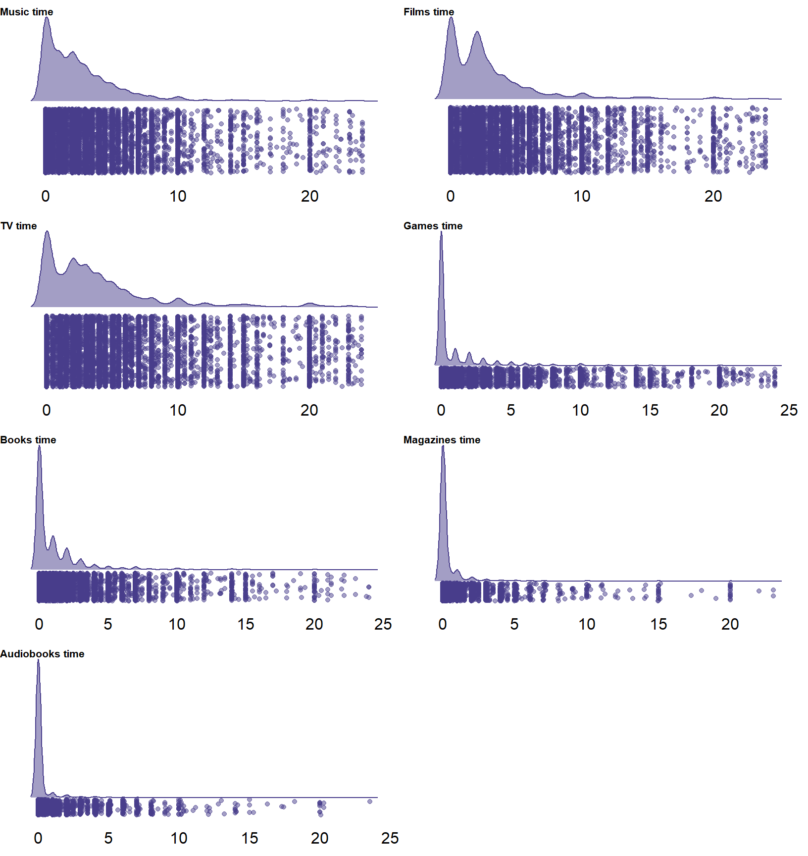
Figure 2.1: Distribution of self-reported time per medium
In Table 2.11 we see that very few entries are above 18h, relative to all other values, which is a good sign.
# count proportion per medium
media_long %>%
  group_by(medium) %>%
  count(time >= 18) %>%
  pivot_wider(
    names_from = `time >= 18`,
    values_from = "n"
  ) %>%
  rename(
    "Below 18h" = `FALSE`,
    "Above 18h" = `TRUE`
  ) %>%
  mutate(
    Proportion = round(`Above 18h` / sum(c(`Above 18h`, `Below 18h`)) * 100, digits = 2)
  ) %>%
  knitr::kable(
    .,
    caption = "Proportion of hours above 18"
)| medium | Below 18h | Above 18h | Proportion |
|---|---|---|---|
| audiobooks | 14165 | 12 | 0.08 |
| books | 14120 | 57 | 0.40 |
| films | 13955 | 222 | 1.57 |
| games | 14025 | 152 | 1.07 |
| magazines | 14158 | 19 | 0.13 |
| music | 14000 | 177 | 1.25 |
| tv | 13775 | 402 | 2.84 |
2.5.1.1 Participant-level
Let’s follow up on those who reported 18h or more use of a medium and check whether there are any participants whose estimates we cannot really trust.
We need to distinguish between completely excluding a participant (whose answers we don’t trust for all waves they provided) and wave-level exclusions (when we trust the data of the participant, except for one or two waves).
As for implausible values on the participant-level, I’d say the following are indicators of poor quality:
- More than 30% of time estimates participants provided (excluding zeros imputed by us) across all waves are above 18h.
- More than one instance of a 23h+ estimate across all waves.
- More than one instance where the sum of nonzero estimates is above 48h in a wave.
Let’s look at the proportion of very high reported use times. Self-reported use is also about how much people feel like they used medium, so I’ll be liberal here. I’d say we can’t trust a participant if they estimated 18+ hours in > 30% of all their time estimates, across all waves. Below, I’ll count per participant how many times they estimated 18+ hours of consumption in relation to all time estimates they provided. I’ll not include zero times in that account because we imputed times of zero.
implausible_pp_level_1  <-
  media_long %>%
  filter(time > 0) %>% # nonzero
  group_by(id, medium) %>%
  summarise(
    above18 = sum(time >= 18),
    below18 = sum(time < 18),
    waves = n()
  ) %>%
  ungroup() %>%
  group_by(id) %>%
  summarise(
    above18 = sum(above18),
    below18 = sum(below18),
    entries = sum(waves),
    proportion_above18 = round(above18 / entries, digits = 2)
  ) %>%
  ungroup() %>%
  arrange(desc(proportion_above18)) %>%
  filter(proportion_above18 > 0.3)

# store the participants that were above that threshold
exclusions_pp_1 <-
  implausible_pp_level_1 %>%
  pull(id) %>%
as.character()| id | above18 | below18 | entries | proportion_above18 |
|---|---|---|---|---|
| pp_103 | 10 | 0 | 10 | 1.00 |
| pp_3009 | 1 | 0 | 1 | 1.00 |
| pp_4833 | 1 | 0 | 1 | 1.00 |
| pp_5153 | 1 | 0 | 1 | 1.00 |
| pp_5468 | 1 | 0 | 1 | 1.00 |
| pp_5915 | 1 | 0 | 1 | 1.00 |
| pp_6008 | 2 | 0 | 2 | 1.00 |
| pp_6610 | 1 | 0 | 1 | 1.00 |
| pp_752 | 5 | 0 | 5 | 1.00 |
| pp_6170 | 4 | 1 | 5 | 0.80 |
| pp_633 | 4 | 1 | 5 | 0.80 |
| pp_6471 | 3 | 1 | 4 | 0.75 |
| pp_128 | 17 | 7 | 24 | 0.71 |
| pp_4394 | 2 | 1 | 3 | 0.67 |
| pp_4446 | 2 | 1 | 3 | 0.67 |
Overall, there were 98 participants who fall into the first exclusion criterion. Next, participants might feel like they played the whole day, so saying 23 hours of play on average is close to impossible. I’d say that can happen, but if it happens twice across waves, I wouldn’t trust that participant.
implausible_pp_level_2 <-
  media_long %>%
  group_by(id) %>%
  summarise(
    above23 = sum(time >= 23),
    below23 = sum(time < 23)
  ) %>%
  filter(above23 > 1)

# store the IDs
exclusions_pp_2 <-
  implausible_pp_level_2 %>%
  pull(id) %>%
as.character()| id | above23 | below23 |
|---|---|---|
| pp_1116 | 3 | 32 |
| pp_1162 | 5 | 37 |
| pp_1246 | 2 | 26 |
| pp_128 | 7 | 35 |
| pp_1420 | 3 | 39 |
| pp_156 | 2 | 19 |
| pp_1737 | 2 | 40 |
| pp_2072 | 2 | 12 |
| pp_2111 | 4 | 38 |
| pp_2287 | 2 | 12 |
| pp_2310 | 2 | 12 |
| pp_2436 | 2 | 40 |
| pp_252 | 5 | 30 |
| pp_2533 | 3 | 39 |
| pp_2537 | 3 | 32 |
By the same logic, some weeks might feel very intense, and participants surely didn’t keep track of what they reported for use throughout all media. So it’s possible if we add up all times, there’ll be instances where the sum is above 24h, even around 48h. After all, participants can multitask, but if they use three media at the same time for 16 hours, that’s 48h. I’d say that can happen theoretically, but not over multiple weeks. So if there’s more than one wave where the total is equal to or above 48h, I don’t think the participant read the question correctly.
# get total time
working_file <-
  working_file %>%
  mutate(
    total_time = rowSums(select(., contains("time")))
  )

# get counts of more than 48h total time
implausible_pp_level_3 <-
  working_file %>%
  group_by(id) %>%
  summarise(
    above48_count = sum(total_time >= 48)
  ) %>%
  filter(above48_count > 1)

# store the IDs
exclusions_pp_3 <-
  implausible_pp_level_3 %>%
  pull(id) %>%
as.character()| id | above48_count |
|---|---|
| pp_1052 | 3 |
| pp_1122 | 5 |
| pp_1162 | 4 |
| pp_128 | 6 |
| pp_13 | 3 |
| pp_1425 | 4 |
| pp_1460 | 6 |
| pp_1510 | 4 |
| pp_1534 | 3 |
| pp_1653 | 4 |
| pp_1655 | 3 |
| pp_1666 | 2 |
| pp_1667 | 4 |
| pp_1688 | 2 |
| pp_1816 | 2 |
Last, let’s check how many unique participants we’d need to exclude if we applied all three of those exclusion criteria (taking into account overalp).
exclusions_pp <-
  c(exclusions_pp_1, exclusions_pp_2, exclusions_pp_3) %>%
  unique()
2.5.1.2 Wave-level
As for implausible values on the wave-level, I’ll apply the following criteria:
- Any wave that has more than two estimates of using a medium for 16h+.
- Any wave where the sum of use times is above 64h.
- Any wave where a participant estimated use of 23h or more.
Again, it’s probably not uncommon to report a high number if I went on a reading-binge. But I’d say if you sleep eight hours, reporting the rest of the time twice for a wave is suspicious, so there’s probably a typo or someone didn’t take the question seriously.
implausible_wave_level_1 <-
  media_long %>%
  group_by(id, wave) %>%
  summarise(
    two16s = sum(time >= 16)
  ) %>%
  filter(two16s > 1)

# store the rows that were above that threshold
exclusions_wave_1 <-
  implausible_wave_level_1 %>%
  select(id, wave)
Overall, we have 166 rows of data we need to exclude from 107 participants. However, of those, 72 were already identified as suspicious in the participant-level exclusions.
Next, we inspect waves where even excessive multitasking per day exceeds a reasonable threshold. If someone multitasked with three media every waking hour, they’d have 16h x 3 = 48h. Therefore, we exclude waves where the sum of use times is equal or above four times all day multitasking: 16h x 3 = 64.
implausible_wave_level_2 <-
  working_file %>%
  mutate(
    total_time = rowSums(select(., contains("time")))
  ) %>%
  filter(total_time >= 64) %>%
  select(id, wave, contains("time"))

# store the rows
exclusions_wave_2 <-
  implausible_wave_level_2 %>%
  select(id, wave)
For this criterion, we have 1026 rows of data we need to exclude from 526 participants. However, of those, 109 were already identified as suspicious in the participant-level exclusions.
Last on the wave-level, we want to exclude any row where participants estimated 23h of daily use of any medium. Maybe one can multitask with three media for 16h a day, but an average use of 23h daily for a week is close to impossible. On the participant level, we already had an exclusion criterion where all of people’s rows were excluded if they had more than one estimate of 23h (across all waves).
implausible_wave_level_3 <-
  media_long %>%
  group_by(id, wave) %>%
  summarise(
    max_time = max(time)
  ) %>%
  filter(max_time >= 23)

# store the rows that were above that threshold
exclusions_wave_3 <-
  implausible_wave_level_3 %>%
  select(id, wave)
For this criterion, we have 184 rows of data we need to exclude from 128 participants. However, of those, 73 were already identified as suspicious in the participant-level exclusions.
Before I remove those cases and rows from the data, I’ll go to response patterns. I’ll do the actual exclusions at the end of this section.
2.5.2 Response patterns
In surveys, people who didn’t take the study seriously often provide implausible values (see section above), rush, or have response patterns. Out of experience, response patterns are an indicator of poor data quality. I’ll mostly be looking at straightlining, so selecting the same answer option for each item in a scale. Usually, straightlining isn’t uncommon for, say, well-being scales, so I don’t want to be too strict here and exclude valid cases.
Also, if participants repeatedly provide the same time estimate across different media, I’d be suspicious of their responses.
- Anyone who straightlined on more than two of the identity scales (minimum of three media).
- Anyone who has the same total time in each wave (minimum three media and waves).
For the first criterion, we calculate the variance for each identity scale (provided participants provided a response). If someone straightlined at three (of at least three) scales, I wouldn’t trust them to take the survey seriously. Note that magazines and audio books didn’t have identity questions.
exclusions_pp_4 <-
  working_file %>%

  # create the variance variables per row
  rowwise() %>%
  mutate(

    # music identity variance
    music_identity_sd = sd(
      c_across(starts_with("music_identity")),
      na.rm = TRUE
    ),

    # films identity variance
    films_identity_sd = sd(
      c_across(starts_with("films_identity")),
      na.rm = TRUE
    ),

    # tv identity variance
    tv_identity_sd = sd(
      c_across(starts_with("tv_identity")),
      na.rm = TRUE
    ),

    # games identity variance
    games_identity_sd = sd(
      c_across(starts_with("games_identity")),
      na.rm = TRUE
    ),

    # epublishing identity variance
    e_publishing_identity_sd = sd(
      c_across(starts_with("e_publishing_identity")),
      na.rm = TRUE
    )
  ) %>%
  unnest(cols = c()) %>%

  # we're only looking at the first wave where the identity questions were asked
  group_by(id) %>%
  filter(wave == 1) %>%
  ungroup() %>%

  # now we check who answered at least three identity scales by summing the filer questions
  mutate(
    media_number = rowSums(select(., filter_music:filter_ebooks)),
    at_least_three = if_else(media_number >= 3, 1, 0)
  ) %>%
  filter(at_least_three == 1) %>%

  # create a variable that counts how many of the variances are zero
  mutate(
    multiple_straightlines = rowSums(select(., ends_with("_sd")) == 0)
  ) %>%
  filter(multiple_straightlines > 2) %>%

  # and select participants
  pull(id) %>%
  as.character()
For this criterion, we have 72 participants. Of those, 6 were already identified as suspicious in the participant-level exclusions previously.
On to the second criterion: Someone might be very consistent and provide the same use times at each wave (excluding nonzero estimates). However, if a person provides the same use estimates for each medium across all waves (minimum three waves), I’d say they’re just trying to get the survey done and rely on the time that they survey prompted.
So below I’ll check who has the same total time (i.e., reporting the same time across all media) in all of their waves. To avoid excluding people for whom this occurred only once, I’ll set a minimum of three media and three waves.
# get participants who have at least three waves and media use estimates
three_media_and_waves <-
  working_file %>%
  mutate(
    media_number = rowSums(select(., starts_with("filter"))) # minimum three media
  ) %>%
  filter(media_number >= 3) %>%
  count(id) %>% # count waves
  filter(n >= 3) %>%
  pull(id) %>%
  as.character()

# then filter by those participants and check how many times their total times are constant
exclusions_pp_5 <-
  working_file %>%
  filter(id %in% three_media_and_waves) %>%
  select(id, wave, total_time) %>%
  group_by(id) %>%
  summarise(
    distinct_times = n_distinct(total_time)
  ) %>%
  filter(distinct_times == 1) %>%
  pull(id) %>%
  as.character()
Only 14 participants fulfilled this criterion. Of those, 1 were already identified as suspicious in the participant-level exclusions previously.
Alright, let’s add those participants with response patterns to those with implausible values.
exclusions_pp <-
  c(exclusions_pp, exclusions_pp_4, exclusions_pp_5) %>%
  unique()
2.5.3 Applying exclusions
As a last step, we exclude those participants whom we identified as having low data quality. How many people we exclude will depend on what our starting sample is. Currently, we still have the whole sample, but for the analysis, we’ll restrict valid cases to those who responded to a certain number of waves.
Below in Table 2.15 I’ll show, per wave, how many people we’d exclude for each exclusion criterion plus what proportion of the valid sample (aka how many participants have at least that many waves) we have left.
Note that some participants fulfill multiple exclusions, so the last columns shows the cumulative exclusions and proportion of the respective sample. For the analysis, mixed-effects models weigh participants with more data more heavily, which means we can use everyone with at least three waves (because we used lagged predictors).| Participants | Wave 1 | Wave 2 | Wave 3 | Wave 4 | Wave 5 | Wave 6 |
|---|---|---|---|---|---|---|
| N | 3863.00 | 2792.00 | 2369.00 | 2132.00 | 1947.00 | 1074.00 |
| Exclusion 1 | 3765.00 | 2764.00 | 2347.00 | 2115.00 | 1931.00 | 1065.00 |
| Exclusion 1 % | 2.54 | 1.00 | 0.93 | 0.80 | 0.82 | 0.84 |
| Exclusion 2 | 3826.00 | 2761.00 | 2343.00 | 2109.00 | 1927.00 | 1061.00 |
| Exclusion 2 % | 0.96 | 1.11 | 1.10 | 1.08 | 1.03 | 1.21 |
| Exclusion 3 | 3810.00 | 2739.00 | 2324.00 | 2093.00 | 1914.00 | 1053.00 |
| Exclusion 3 % | 1.37 | 1.90 | 1.90 | 1.83 | 1.69 | 1.96 |
| Exclusion 4 | 3791.00 | 2739.00 | 2324.00 | 2092.00 | 1911.00 | 1055.00 |
| Exclusion 4 % | 1.86 | 1.90 | 1.90 | 1.88 | 1.85 | 1.77 |
| Exclusion 5 | 3849.00 | 2778.00 | 2355.00 | 2120.00 | 1935.00 | 1068.00 |
| Exclusion 5 % | 0.36 | 0.50 | 0.59 | 0.56 | 0.62 | 0.56 |
| Exclusion all | 3630.00 | 2648.00 | 2246.00 | 2027.00 | 1853.00 | 1022.00 |
| Exclusion all % | 6.03 | 5.16 | 5.19 | 4.92 | 4.83 | 4.84 |
Let’s also combine all wave-level exclusions.
# first, I'll combine all three wave-level exclusions
exclusions_wave <-
  full_join(
    exclusions_wave_1,
    exclusions_wave_2
  ) %>%
  full_join(
    .,
    exclusions_wave_3
  ) %>%
  ungroup() %>%
  distinct()
Before we apply the exclusions, let’s first create a data frame which we can use later to plot exclusions for the paper. It’ll be similar to the one above, but restricted to those with at least three waves, because those are the ones we ultimately use for the analysis. The code below might duplicate some of the work of previous and later code, but I came back here for creating a plot for the paper, so I didn’t want to break anything.
# vectors holding number of participants and number of observations
PPs <- c()
Observations <- c()

# temp data set of people with at least three waves
dat <-
  working_file %>%
  group_by(id) %>%
  filter(n() >= 3) %>%
  ungroup()

# the exclusions we iterate over
exclusions <-
  list(
    exclusions_pp_1,
    exclusions_pp_2,
    exclusions_pp_3,
    exclusions_pp_4,
    exclusions_pp_5,
    exclusions_wave_1,
    exclusions_wave_2,
    exclusions_wave_3
  )

# iterate over each exclusion criterion list/tibble and extract how many are left after excluding those
for (i in exclusions) {
  if(!is_tibble(i)){
    PPs <- c(PPs, dat %>% filter(!id %in% i) %>% summarise(PPs = length(unique(id))) %>% pull(PPs))
    Observations <- c(Observations, dat %>% filter(!id %in% i) %>% summarise(n = n()) %>% pull(n))
  } else{
    PPs <-
      c(
        PPs,
        anti_join(
          dat,
          i
        ) %>%
          summarise(PPs = length(unique(id))) %>%
          pull(PPs)
      )
    Observations <-
      c(
        Observations,
        anti_join(
          dat,
          i
        ) %>%
          summarise(n = n()) %>%
          pull(n)
      )
  }
}

# our data for the plot
exclusion_plot_data <-
  tibble(
    "Type" = c(rep("Participant-level", 5), rep("Wave-level", 3), "Total", "Total Before"),
    "Exclusion" = c(1:5, 1:3, "Total", "Total Before"),
    "PPs" = c(
      PPs,
      dat %>%
        filter(!id %in% exclusions_pp) %>%
        anti_join(
          .,
          exclusions_wave
        ) %>%
        group_by(id) %>%
        filter(n() >= 3) %>%
        ungroup() %>%
        summarise(
          n = length(unique(id))
        ) %>%
        pull(n),
      length(unique(dat$id))
    ),
    "Observations" = c(
      Observations,
      dat %>%
        filter(!id %in% exclusions_pp) %>%
        anti_join(
          .,
          exclusions_wave
        ) %>%
        group_by(id) %>%
        filter(n() >= 3) %>%
        ungroup() %>%
        summarise(
          n = n()
        ) %>%
        pull(n),
      nrow(dat)
    )
  )

# clear workspace
rm(PPs, Observations, exclusions, dat)
Let’s apply participant-level exclusions.
# exclusions_pp contains all participant-level exclusions
working_file <-
  working_file %>%
  filter(!id %in% exclusions_pp)
Now that we’ve applied the participant-level exclusions, we also need to take a look at wave-level exclusions. It’s quite possible that having excluded participants with low-quality data already excluded many of their low-quality rows as well.
I’ll check how many rows that we intended to exclude on the wave-level are already not in the data set anymore because the entire participant that row belongs to was excluded during participant-level exclusions.
anti_join(
  exclusions_wave,
  working_file,
  by = c("id", "wave")
) %>%
  nrow()
## [1] 385Let’s take the data set after participant exclusions, exclude low-quality rows (i.e., waves) and count the number of waves again.
Table 2.16 shows the number of participants with at least a number of waves (after participant-level exclusions) next to the same number after excluding on the wave-level. The sharpest drop is in the number of people who previously had completed six waves. That’s not surprising because each unique participant inexclusions_wave (553 participants) who had previously completed six waves now drops down to five waves.
Probably there’s a correlation between sticking around for this long and motivation, such that motivation drops in later waves and there’s a higher chance to fulfill one of the exclusion criteria.
Overall, 5.13% of rows are excluded.
| Waves | Participants per wave | Participants per wave after exclusions | Reduction proportion % |
|---|---|---|---|
| 1 | 3630 | 3513 | 3.22 |
| 2 | 2648 | 2557 | 3.44 |
| 3 | 2246 | 2159 | 3.87 |
| 4 | 2027 | 1921 | 5.23 |
| 5 | 1853 | 1704 | 8.04 |
| 6 | 1022 | 883 | 13.60 |
During model fitting, we’ll predict the outcome with the lagged value of the predictor. If we merely exclude the rows participants will have gaps in their waves. For example, a participant might have entries for waves 1-4, but wave 3 belongs to low-quality data rows. We’d then be left with rows 1,2, and 4. During model fitting, just lagging the value would mean the outcome at wave 4 is predicted by the predictor at wave 2 - effectively messing up our one-week lag between waves.
Therefore, it makes sense to maintain those rows whose data we exclude, but set them to NA.
This way, we don’t have “gaps” between waves.
In addition, if we want to impute missing values during model fitting (via the built-in brms imputation), we want to be able to know what value to impute, which is why we need the NA signal.
Let’s make those rows that have low quality data, then set all wave-level entries to NA on those rows.
# add marker to wave-level exclusions
exclusions_wave <-
  exclusions_wave %>%
  mutate(set_to_na = 1)

# add that marker to working file
working_file <-
  left_join(
    working_file,
    exclusions_wave,
    by = c("id", "wave")
  )

# then set all wave-level entries to NA that have a marker
working_file <-
  working_file %>%
  mutate(
    across(
      c(
        music_hours:well_being_2,
        music_time:total_time
      ),
      ~ replace(.x, set_to_na == 1, NA)
    )
  ) %>%
  # remove marker
  select(-set_to_na)
2.6 Build scales
As a last step, we’re creating the mean score scales.
Before we do that, we have to reverse code some items.
identity items had strongest agreement as 1.
I find it more intuitive when larger numbers mean more agreement.
The same applies to the well-being item about anxiety, which I will reverse code.
working_file <-
  working_file %>%
  mutate(
    across(
      contains("identity"),
      ~ 5 - .x
    ),

    well_being_2 = 10 - well_being_2 # starts at 0
  )
Let’s start with the identity scales; for each medium (except magazines and audiobooks), participants indicated how much that medium was part of their identity.
working_file <-
  working_file %>%
  mutate(

    # music
    music_identity = rowMeans(select(., starts_with("music_identity"))),

    # films
    films_identity = rowMeans(select(., starts_with("films_identity"))),

    # tv
    tv_identity = rowMeans(select(., starts_with("tv_identity"))),

    # games
    games_identity = rowMeans(select(., starts_with("games_identity"))),

    # epublishing
    e_publishing_identity = rowMeans(select(., starts_with("e_publishing_identity"))),
  )
And the well-being scales per wave (aka row).
working_file <-
  working_file %>%
  mutate(
    life_satisfaction = rowMeans(select(., starts_with("life_satisfaction"))),
    affect = rowMeans(select(., starts_with("well_being"))),
    well_being = rowMeans(select(., starts_with("well_being"), starts_with("life_satisfaction"))) # both affect and well-being combined
  )
Before we move on to visualizations and descriptive info, I’ll do some housekeeping. I’ll reorder some variables for cosmetic purposes, only select those we need, and clean the workspace.
# select relevant variables
working_file <-
  working_file %>%
  select(
    id,
    gender,
    wave:filter_audiobooks,
    starts_with("music"),
    starts_with("films"),
    starts_with("tv"),
    starts_with("games"),
    starts_with("e_publishing"),
    starts_with("books"),
    starts_with("magazines"),
    starts_with("audiobooks"),
    total_time,
    starts_with("life_satisfaction"),
    starts_with("well_being"),
    affect,
    -ends_with("hours"), # we got the total time from here on
    -ends_with("minutes"),
  )

# clean workspace
rm(
  markers,
  no_changes,
  waves_per_id,
  an_id,
  id_counter,
  id_to_match,
  ids,
  temp_id,
  three_media_and_waves
)
Before I remove those who only have three waves, I’ll create a temporary working file that we use in the next chapter to look at demographics per number of filled out surveys.
temp <- working_fileAnd then remove those who don’t have at least three waves. For one model part, we’ll used led values, so two waves won’t be enough because that means a participant is left with only one wave once we lead a predictor.
Also, some participants now have missing values (because we applied the wave-level exclusions).
Missing values will be removed during model fitting, meaning that if someone has three waves, but two of them are NA, they’ll be left with one wave of data.
So I’ll filter the data set to only keep those with at least three waves with responses.
# get ids of participants who have at least three valid waves
at_least_three <-
  working_file %>%
  group_by(id) %>%
  filter(!is.na(music_time)) %>%
  filter(n() >= 3) %>%
  ungroup() %>%
  pull(id)

# then only keep those participants
working_file <-
  working_file %>%
  filter(id %in% at_least_three)

# remove from workspace
rm(at_least_three)