4 Analysis
Our overarching research question is how media use in different categories and well-being influence each other over time. There were four well-being items; two were asking about life in general, two about affective states yesterday. I don’t think, just based on face validity, that these four items form one concept, which is why I treated them separately in the data processing.
Let’s run a confirmatory factor analysis on the first wave and inspect the fit. The fit is poor-ish and the model suggest that we should correlate the residuals of the life satisfaction items with each other and of the affect items with each other.
That confirms my idea about treating those four items as coming from two different constructs.
cfa_model <-
  "well_being_factor =~ life_satisfaction_1 + life_satisfaction_2 + well_being_1 + well_being_2"

# get fit
cfa_fit <- cfa(
  cfa_model,
  data = working_file %>%
    filter(wave == 1)
)

# inspect summary
summary(
  cfa_fit,
  fit.measures = TRUE,
  modindices = TRUE
)
## lavaan 0.6-7 ended normally after 25 iterations
##
## Estimator ML
## Optimization method NLMINB
## Number of free parameters 8
##
## Used Total
## Number of observations 2103 2159
##
## Model Test User Model:
##
## Test statistic 152.823
## Degrees of freedom 2
## P-value (Chi-square) 0.000
##
## Model Test Baseline Model:
##
## Test statistic 4689.433
## Degrees of freedom 6
## P-value 0.000
##
## User Model versus Baseline Model:
##
## Comparative Fit Index (CFI) 0.968
## Tucker-Lewis Index (TLI) 0.903
##
## Loglikelihood and Information Criteria:
##
## Loglikelihood user model (H0) -16789.925
## Loglikelihood unrestricted model (H1) -16713.513
##
## Akaike (AIC) 33595.849
## Bayesian (BIC) 33641.058
## Sample-size adjusted Bayesian (BIC) 33615.641
##
## Root Mean Square Error of Approximation:
##
## RMSEA 0.189
## 90 Percent confidence interval - lower 0.165
## 90 Percent confidence interval - upper 0.215
## P-value RMSEA <= 0.05 0.000
##
## Standardized Root Mean Square Residual:
##
## SRMR 0.038
##
## Parameter Estimates:
##
## Standard errors Standard
## Information Expected
## Information saturated (h1) model Structured
##
## Latent Variables:
## Estimate Std.Err z-value P(>|z|)
## well_being_factor =~
## life_stsfctn_1 1.000
## life_stsfctn_2 0.952 0.019 51.334 0.000
## well_being_1 1.012 0.018 54.730 0.000
## well_being_2 0.575 0.032 18.148 0.000
##
## Variances:
## Estimate Std.Err z-value P(>|z|)
## .life_stsfctn_1 0.764 0.047 16.108 0.000
## .life_stsfctn_2 1.413 0.058 24.476 0.000
## .well_being_1 1.156 0.055 20.862 0.000
## .well_being_2 6.871 0.216 31.883 0.000
## well_beng_fctr 3.740 0.143 26.163 0.000
##
## Modification Indices:
##
## lhs op rhs mi epc sepc.lv sepc.all sepc.nox
## 10 life_satisfaction_1 ~~ life_satisfaction_2 147.866 1.518 1.518 1.461 1.461
## 11 life_satisfaction_1 ~~ well_being_1 49.432 -1.025 -1.025 -1.090 -1.090
## 12 life_satisfaction_1 ~~ well_being_2 29.103 -0.381 -0.381 -0.166 -0.166
## 13 life_satisfaction_2 ~~ well_being_1 29.103 -0.639 -0.639 -0.500 -0.500
## 14 life_satisfaction_2 ~~ well_being_2 49.432 -0.554 -0.554 -0.178 -0.178
## 15 well_being_1 ~~ well_being_2 147.867 0.928 0.928 0.329 0.3294.1 Data preparation
We’re interested in reciprocal effects of media use and well-being. Usually, I’d go for Random-Intercept Cross-Lagged Panel Models (RICLPM), but we have such massive zero inflation that the distribution of media use might bias the results.
I emailed one of the co-authors of the Random-Intercept Cross-Lagged Panel Models and he said that these models are only well-understood for normally distributed data. Absent any simulation studies that show that these models can retrieve parameters from a non-normal data generating process, I’ll look for an alternative.
Instead, I’ll rely on a mixed-models framework. Per well-being outcome (so affect and life satisfaction) and medium, I’ll run two models:
- The first model predicts well-being from lagged media use. We can treat well-being as normally distributed.
- The second mode predicts media use from lagged well-being. We treat media use as zero-inflated with a gamma distribution.
These models have the advantage that we don’t need to impute missing waves. Instead, the model will weigh those with more data more heavily for the outcome distribution. Because we use lagged predictors in the model predicting use, a participant must have at least three valid waves. When we lag, the model will automatically exclude the first wave (because half of its information is contained in the second wave now). Some participants also have missing values on some waves - which is why we only kept those participants with at least three rows of data. So someone with all six waves but four excluded waves will not be included in the final sample.
For both types of models, we’ll separate between- and within-person effects. We’ll not control for the lagged value of the dependent variable, see here.
To be able to distinguish between within- and between-person effects, we’ll need to make use of centering. We’re dividing each predictor into a stable, level-2 (person-level) component, and a component that tells us how much each measurement deviates from that stable component (level-1 or within-person effect). See instructions from this excellent blog post.
working_file <-
  working_file %>%
  group_by(id) %>%
  mutate(
    across(
      c(
        affect,
        life_satisfaction,
        ends_with("time")
      ),
      list(
        between = ~ mean(.x, na.rm = TRUE),
        within = ~ .x - mean(.x, na.rm = TRUE)
      )
    )
  ) %>%
  ungroup()
Also, we’re interested in the threshold of going from not using a medium to using a medium. This is due to how the media use variable is distributed: Lots of zeros and continuous if not zero. Because of how we treated zeros so far, we know that zeros are qualitatively different from nonzeros. Zero means not having used at all (possibly a different process), nonzero means how much you used a medium if you used it.
When media use is the outcome variable, we’ll model those different processes with a zero-inflation distribution. It’s my understanding that it’s not a good idea to select an outcome distribution based on the histogram of a variable. Richard McElreath calls this “histomancy.” After all, it’s about the distribution of the residuals after model fitting - so a weird looking distribution might still be the result of a normally distributed data generating process. In our case, I think the use variable doesn’t come from a normally distributed data generating process because we know that using vs. not using a medium is a different process. Likewise, we know that if someone used a medium, their use time cannot be zero and will be skewed toward lower values, with fewer and fewer larger values as use increases. That’s a typical case for a Gamma distribution.
When media use is the predictor, we need to tell the model that there’s something special about zeros or not zeros. That’s why we’ll include a new indicator variable for whether use is zero or not. See this discussion.
In this discussion, they talk about a case where there’s only one observation per case. However, I want to distinguish within- and between-person effects, like I did with the continuous part of use time. I’ll match that strategy with the indicator.
First, per medium and wave, I’ll create an index variable that’s 1 when someone used a medium for a wave, and 0 when not. Second, I’ll take the average of that index variable per person. That gives us a between-person proportion. The parameter for that proportion will tell us what happens for well-being if we compare nonusers (0 proportion) to users (100 proportion), so if we go from 0 to 1. Third, we center each participant’s rows with that proportion, just like we did with use time. The parameter for this variable tells us what happens within a person when they go from not using to using, so if we go from their average to their average plus one.
For example, suppose someone listened to music in three of the six waves. They’ll have their average time as the between-person effect and their deviation from that average time as the within-person effect. That’s what we did with the centering above. That person will therefore have a constant proportion of having listened to music (yes or no) of 50%. The parameter for this variable will then tell us what happens if we go one up on the proportion scale, which is bound at [0|1]. In other words, if there’s someone else who listened to music in 67% of waves, the model will give us a parameter for a comparison of not using (0) to using (1), based on all the proportion between people. Strictly speaking, the model will tell us what happens if the proportion increases by one, but we can interpret this increase as going from nonuse to use because the proportion is bound at those values.
As for the within-part, say the first person listened to music every other wave.
Their within-indicator would then take the values of used (1 or 0) minus proportion of use (0.5) = c(-0.5, 0.5, -0.5, 0.5, -0.5, 0.5) for the six waves.
The parameter for that indicator would tell us what happens if a user goes up one point above their average proportion of listening to music across all waves.
But this proportion is bound at [0|1], so effectively this tells us what happens if the user goes from not listening to music to listening to music (aka 1 up) because the raw scores are always 0 or 1.
I’ll create this index variable and center it like I did above.
Note that we already have filter variables, but those refer to whether someone used a medium in the three months before the first wave.
That’s why I’ll use the used suffix here.
working_file <-
  working_file %>%
  mutate(
    across(
      c(
        ends_with("time"),
        -total_time
      ),
      list(
        used = ~ if_else(.x == 0, 0, 1)
      )
    )
  ) %>%

  # remove the _time part of the variable name
  rename_with(
    ~ str_remove(.x, "time_"),
    ends_with("used")
  ) %>%

  # center those variables
  group_by(id) %>%
  mutate(
    across(
      ends_with("used"),
      list(
        between = ~ mean(.x, na.rm = TRUE),
        within = ~ .x - mean(.x, na.rm = TRUE)
      )
    )
  )
We had NAs for those who had poor quality data in a row.
However, when introducing the between variables above, we assigned a constant per participant, overwriting the NA.
So I’ll reintroduce NA on the between and used variables.
I’ll condition on a random variable that’s NA - affect in this case..
Any other variable would also work because all wave-level entries will be NA.
working_file <-
  working_file %>%
  mutate(
    across(
      c(
        contains("used"),
        contains("between")
      ),
      ~ replace(.x, is.na(affect), NA)
    )
  )
Last, we need to create the lagged and led variables.
If we add them to the model as lag(variable)/lead(variable), it will merely shift values one up/down across all participants.
But we need to lag/lead for each participant.
We can do that when specifying the data, but that’s prone to error with that many models.
So I’ll manually create lagged/led variables in our working file where we lag/lead per participant.
Note that we don’t need to lag everything here: The data are “naturally” lagged. At each wave, participants reported their average daily use of a medium for the preceding week and their current well-being. So lagging the times variable would mean we’re predicting current well-being with the reports of use from last week, which themselves refer to the week before. Therefore, we don’t need to lag the time variables - they are lagged already. The same holds for variables that show whether someone used a medium or not. They’re also referring to the previous week, so are “naturally” lagged.
As for the well-being indicators: Here we don’t want to lag the variable, but lead them. Affect at wave 1 should predict use and time at wave 2, so we need to “move down” use and time one row per participant. Obviously, lagging well-being or leading use is the same, but I find leading more intuitive here because it corresponds to the time line of the data.
working_file <-
  working_file %>%
  group_by(id) %>%
  mutate(
    across(
      c(
        ends_with("_time")
      ),
      lead,
      .names = "lead_{.col}"
    )
  ) %>%
  ungroup()
Note, I saved all brms model objects and load them below.
Each model takes quite some time and the files get huge (a total of 35GB).
If you’re reproducing the analysis and don’t want to run the models yourself, you can download the model objects from the OSF.
For that, you need to set the code chunk below to eval=TRUE, which creates a model/ directory with all models inside.
# create directory
dir.create("models/", FALSE, TRUE)

# download models
osf_retrieve_node("https://osf.io/yn7sx/?view_only=2d0d8bf4850d4ace8a08c860bc45e9f2") %>%
  osf_ls_nodes() %>%
  filter(name == "models") %>%
  osf_ls_files(
    .,
    n_max = Inf
  ) %>%
  osf_download(
    .,
    path = here("models"),
    progress = TRUE
  )
Last, I’ll write that data object into the data folder now that we have our final analysis data file.
write_rds(working_file, here("data", "processed_data.rds"))4.2 Music
4.2.1 Affect
4.2.1.1 Music on affect
Let’s begin with modeling affect and music over time. In addition to separating within and between effects, we also let the within effects vary. So the fixed effects tell us how much an average person changed on well-being a week later if they went from not using to using a medium and how much well-being changed if a person used a medium an hour more than they usually do. We allow both of those effects to vary across participants.
music_affect <-
  brm(
    data = working_file,
    family = gaussian,
    affect ~
      1 +
      music_used_between +
      music_used_within +
      music_time_between +
      music_time_within +
      (1 +
         music_time_within +
         music_used_within
       | id),
    iter = 5000,
    warmup = 2000,
    chains = 4,
    cores = 4,
    seed = 42,
    control = list(adapt_delta = 0.95),
    file = here("models", "music_affect")
  )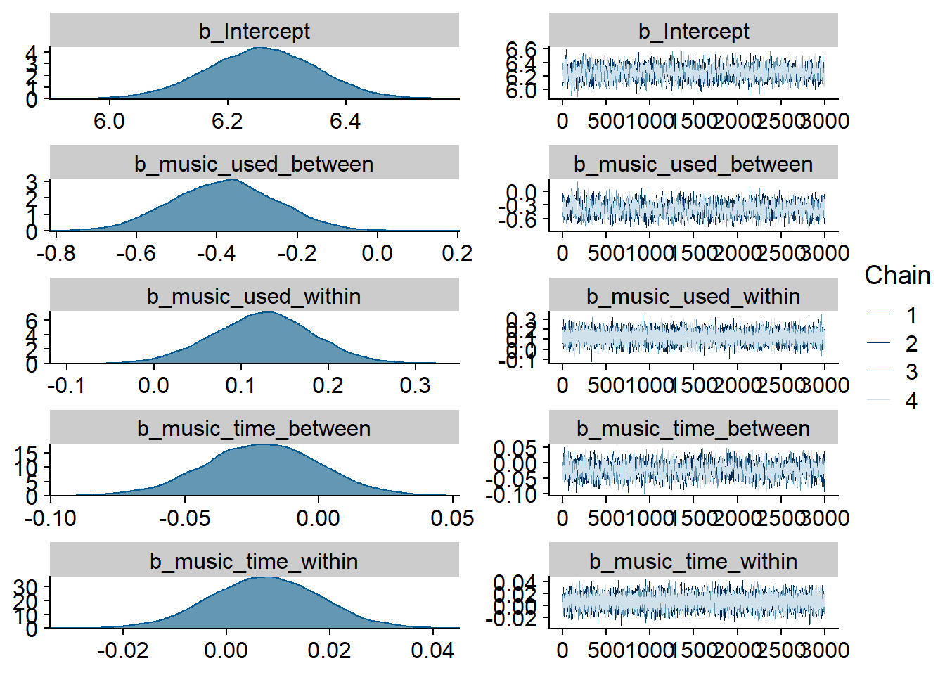
Figure 4.1: Traceplots and posterior distributions for Music-Affect model
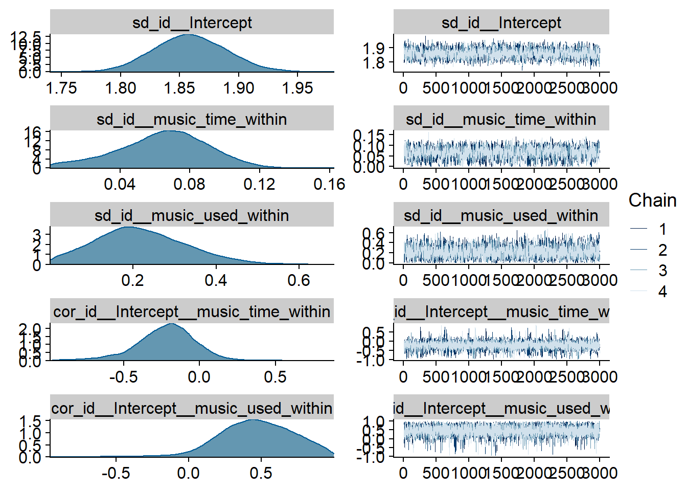
Figure 4.2: Traceplots and posterior distributions for Music-Affect model
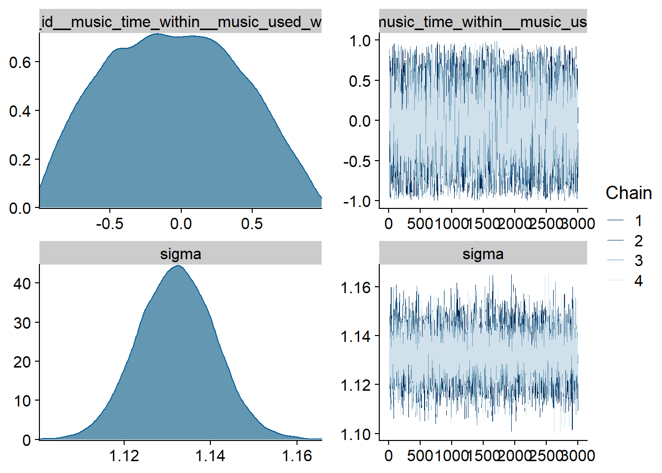
Figure 4.3: Traceplots and posterior distributions for Music-Affect model
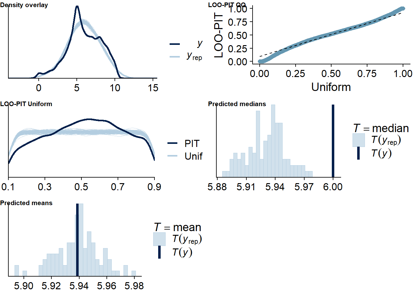
Figure 4.4: Posterior predictive checks for Music-Affect model
Let’s also check for potentially influential values. Quite a lot are flagged: This might have to do with the fact that some participants only had three observations. If we leave one out, the posterior will be influenced heavily by the two remaining observation, see the discussion here. Unfortunately, using moment matching to get better LOO estimates doesn’t work for me, even when I save all parameters. Apparently, this could be a bug. And calculating ELPD directly isn’t an option because it would take days.
Overall, I’m inclined to trust the model (conditional on us using a normal outcome distribution) because of the model diagnostics. It’s possible that some of the larger values on the time variable (which are quite rare) have a large influence on the posterior if they come from the same person. But we already excluded many implausible values, so this is the sample we’re working with and from which we want to generalize to the population.
music_affect_loo <- loo(music_affect)
music_affect_loo
##
## Computed from 12000 by 10985 log-likelihood matrix
##
## Estimate SE
## elpd_loo -18112.0 105.4
## p_loo 1955.7 34.5
## looic 36224.0 210.8
## ------
## Monte Carlo SE of elpd_loo is NA.
##
## Pareto k diagnostic values:
## Count Pct. Min. n_eff
## (-Inf, 0.5] (good) 10617 96.6% 434
## (0.5, 0.7] (ok) 330 3.0% 93
## (0.7, 1] (bad) 36 0.3% 28
## (1, Inf) (very bad) 2 0.0% 19
## See help('pareto-k-diagnostic') for details.Let’s inspect the summary. We see that:
- Music listeners were less happy than those who didn’t listen to music (
music_used_between). The model also estimates the effect to be quite large: listeners scored 0.38 points lower on the ten-point scale. The credible interval doesn’t include zero, so conditional on the model, the data are 95% likely to have been generated by a true effect that does not include zero. - However, if a person went from not listening to listening, they felt better the next week (
music_used_within). That effect is smaller than the between effect: If someone stopped listening they felt 0.12 points worse. The credible interval doesn’t contain zero, but barely. - When a person listened to one hour more music than someone else, that person also felt slightly worse (
music_time_between). However, the effect is small and the posterior contains zero as well as positive effects, so we can’t be certain. - The same goes for a one-hour increase from one’s typical music listening (
music_time_within): the effect is positive, but super small and the posterior contains zero as well as negative values.
summary(music_affect)## Family: gaussian
## Links: mu = identity; sigma = identity
## Formula: affect ~ 1 + music_used_between + music_used_within + music_time_between + music_time_within + (1 + music_time_within + music_used_within | id)
## Data: working_file (Number of observations: 10985)
## Samples: 4 chains, each with iter = 5000; warmup = 2000; thin = 1;
## total post-warmup samples = 12000
##
## Group-Level Effects:
## ~id (Number of levels: 2159)
## Estimate Est.Error l-95% CI u-95% CI Rhat Bulk_ESS Tail_ESS
## sd(Intercept) 1.86 0.03 1.80 1.92 1.00 2558 5066
## sd(music_time_within) 0.06 0.03 0.01 0.11 1.00 1546 1804
## sd(music_used_within) 0.22 0.11 0.03 0.45 1.00 3101 3835
## cor(Intercept,music_time_within) -0.22 0.21 -0.68 0.15 1.00 6556 3633
## cor(Intercept,music_used_within) 0.46 0.26 -0.07 0.92 1.00 7058 6344
## cor(music_time_within,music_used_within) -0.05 0.46 -0.87 0.79 1.00 4688 6431
##
## Population-Level Effects:
## Estimate Est.Error l-95% CI u-95% CI Rhat Bulk_ESS Tail_ESS
## Intercept 6.26 0.09 6.07 6.44 1.00 2009 3590
## music_used_between -0.38 0.13 -0.63 -0.12 1.00 1849 3799
## music_used_within 0.12 0.06 0.01 0.24 1.00 24236 9993
## music_time_between -0.02 0.02 -0.06 0.02 1.00 1988 3865
## music_time_within 0.01 0.01 -0.01 0.03 1.00 19482 10123
##
## Family Specific Parameters:
## Estimate Est.Error l-95% CI u-95% CI Rhat Bulk_ESS Tail_ESS
## sigma 1.13 0.01 1.11 1.15 1.00 9868 9496
##
## Samples were drawn using sampling(NUTS). For each parameter, Bulk_ESS
## and Tail_ESS are effective sample size measures, and Rhat is the potential
## scale reduction factor on split chains (at convergence, Rhat = 1).used effects have less uncertainty associated with the extreme ends of the distribution, whereas time effects have a lot of uncertainty around smaller and larger values, probably because there aren’t many data points here.
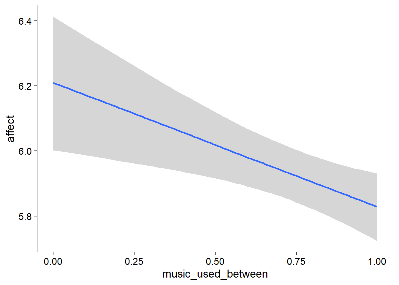
Figure 4.5: Conditional effects for Music-Affect model
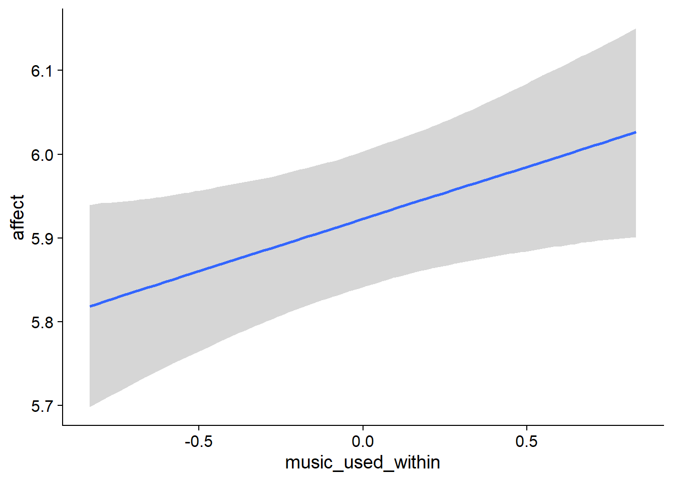
Figure 4.6: Conditional effects for Music-Affect model
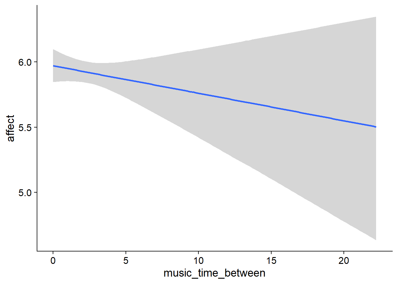
Figure 4.7: Conditional effects for Music-Affect model
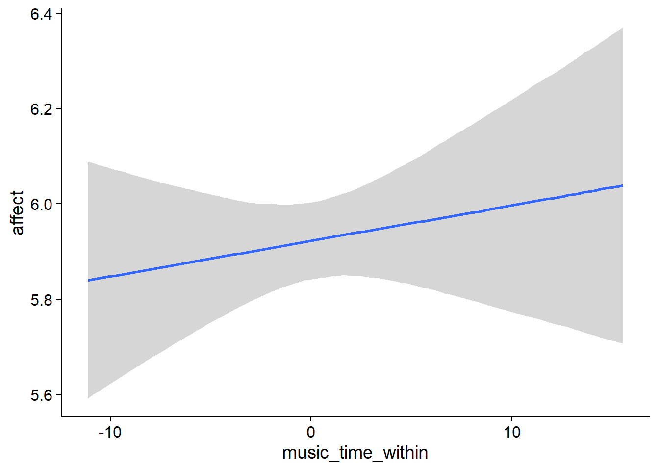
Figure 4.8: Conditional effects for Music-Affect model
##            used  (Mb) gc trigger   (Mb)  max used   (Mb)
## Ncells  3690040 197.1    6044351  322.9   6044351  322.9
## Vcells 23760528 181.3  147626532 1126.4 176402606 1345.9
4.2.1.2 Affect on music
Let’s do the other lag of the model: The effect of affect in the previous week on music listening. Here, we’ll use a zero-inflated gamma distribution. The zero-inflation is obvious: Not everyone uses each medium at each wave. Like I said above, that’s a clear argument that zero vs. not zero is a different data generating process than time listened.
And like above, where I wanted to see how listening vs. not listening is related to affect a week later, I want to see whether changes in affect are related to changes in the probability to listen to music a week later. Besides predicting listening vs. not listening, we also want to see whether changes in affect are related to changes in music listening duration a week later (so the non-zero parts of media use). We know that the non-zero duration is continuous (i.e., hours) and cannot be zero. We can also see from the distribution that the variation increases with larger values, so the variation likely increases with the mean. That’s why I think a Gamma distribution is adequate.
Below I run the model. Note again that music time is naturally lagged (i.e., reported for the previous week). So get the lagged effect of affect on music time, we use the led music time.
On my machine, the model took about an two hours.
affect_music <-
  brm(
    bf(
      # predicting continuous part
      lead_music_time ~
        1 +
        affect_between +
        affect_within +
        (1 +
           affect_within
         | id),

      # predicting hurdle part
      hu ~
        1 +
        affect_between +
        affect_within +
        (1 +
           affect_within
         | id)
    ),
    data = working_file,
    family = hurdle_gamma(),
    ,
    iter = 5000,
    warmup = 2000,
    chains = 4,
    cores = 4,
    seed = 42,
    control = list(adapt_delta = 0.95),
    file = here("models", "affect_music")
  )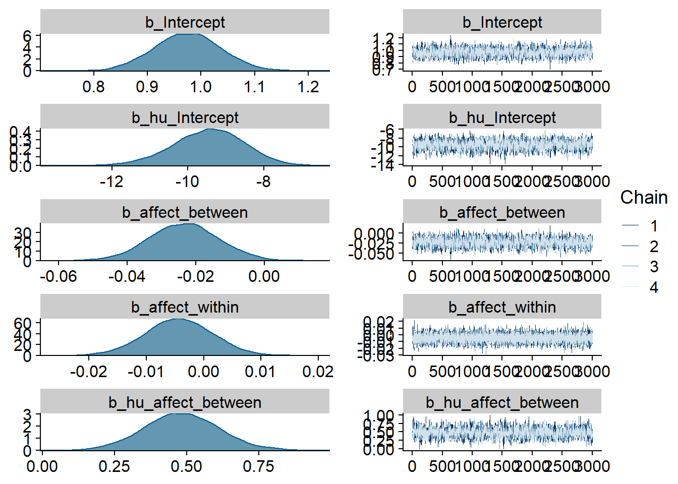
Figure 4.9: Traceplots and posterior distributions for Affect-Music model
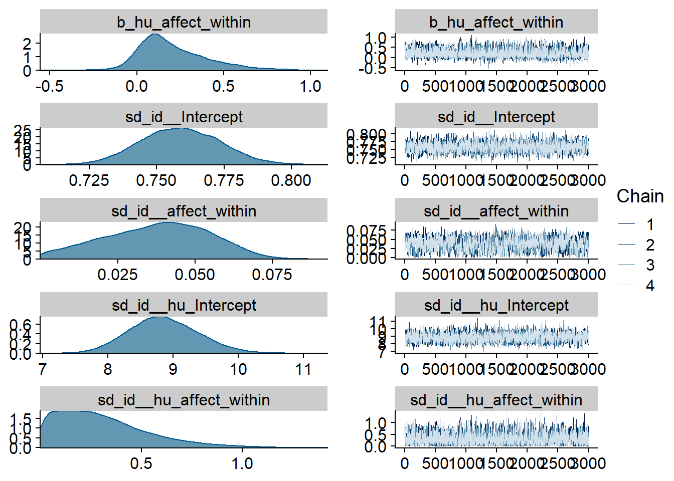
Figure 4.10: Traceplots and posterior distributions for Affect-Music model
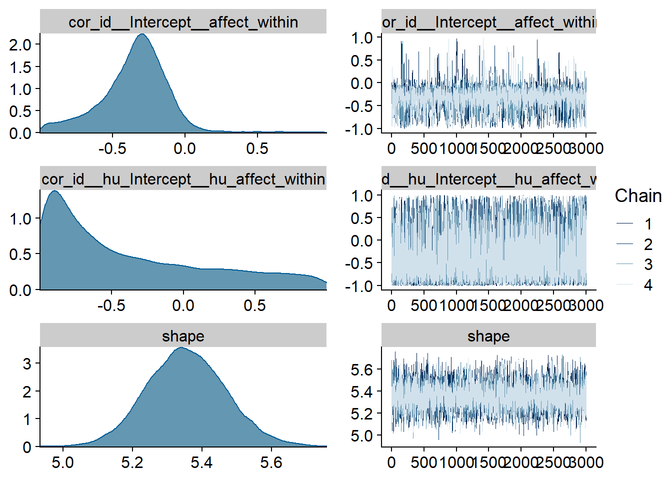
Figure 4.11: Traceplots and posterior distributions for Affect-Music model
The posterior predictive distribution (Figure 4.12) shows that the model does an excellent job in predicting our outcome - at least if we follow the distribution. Self-reported time will necessarily bundle around full and half hours (e.g., 0.5h, 1h, 1.5h etc.), which is why the distribution of the data has spikes. The model smooths those spikes, which is a good thing because we want to get at the data generating process.
It retrieves the mean well, but underestimates the median, quite possibly because the model expects less zeros, but more very small values - which is what we want from multilevel models: shrinkage. The other model fit diagnostics are okay, but not great.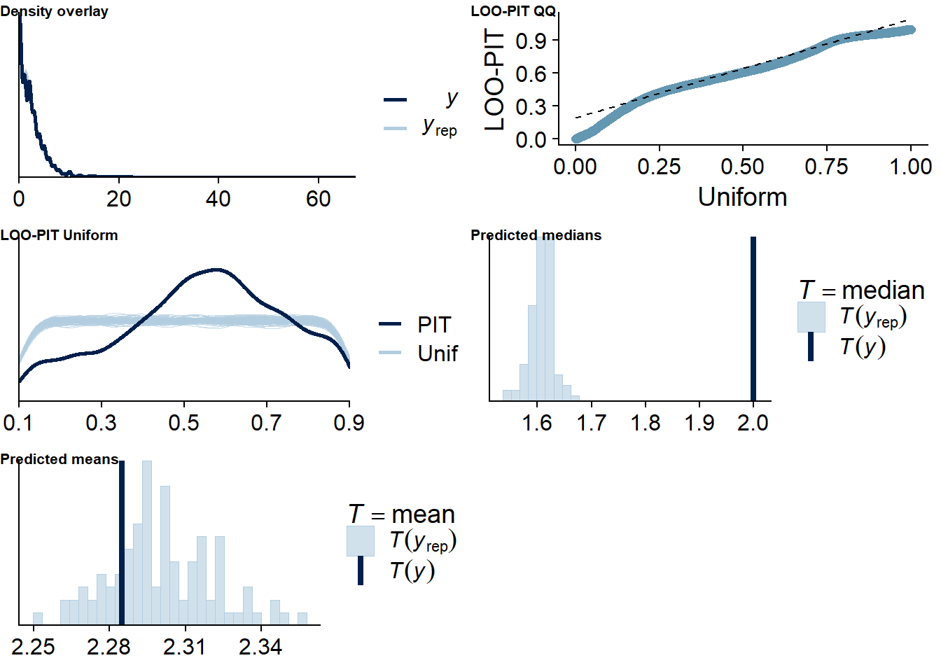
Figure 4.12: Posterior predictive checks for Affect-Music model
Let’s also check for potentially influential values. A lot are flagged, like in the previous model: Again, I think that speaks for the flexibility of the model. There are multiple participants with only two observations. If we leave one out, the posterior will be influenced heavily by the one remaining observation Once more, I’m inclined to trust the model because the model diagnostics looked good.
affect_music_loo <- loo(affect_music)
affect_music_loo
##
## Computed from 12000 by 8698 log-likelihood matrix
##
## Estimate SE
## elpd_loo -11519.8 123.4
## p_loo 2101.0 53.1
## looic 23039.6 246.8
## ------
## Monte Carlo SE of elpd_loo is NA.
##
## Pareto k diagnostic values:
## Count Pct. Min. n_eff
## (-Inf, 0.5] (good) 7702 88.5% 761
## (0.5, 0.7] (ok) 630 7.2% 100
## (0.7, 1] (bad) 264 3.0% 10
## (1, Inf) (very bad) 102 1.2% 1
## See help('pareto-k-diagnostic') for details.Summary:
- For
muwe’re on the log scale, so we need to exponentiate which yieldsexp(0.97)= 2.64 hours on non-zero music time - when a participant has zero affect and no deviation from that affect, so not a very meaningful number (Intercept) - For the hurdle, so the odds of having zero rather than not zero, the model estimates considerable shrinkage: The probability of having a zero is
plogis(-9.46)= 7.7900522^{-5}, much smaller than the proportion of zeros in the actual data. That’s okay, because most zeros come from very few participants who have all zero, so the model takes that into account (hu_Intercept). - When we look at the effect of affect on non-zero hours, we’re still on the log scale, meaning we need to exponentiate which gives us the factor at which y increases with each increase on x: If we compare a participant with another participant with an increase of one on affect, their music time increases (so decreases) by a factor of
exp(-0.02)= 0.98 one week later - a small effect, but the posterior doesn’t include zero (affect_between) - The same goes for the within effect: As a person goes up one point on affect compared to their typical affect score, their music time increases (i.e., decreases) by a factor of
exp(-0.004)= 1 - a completely negligible, small effect whose posterior includes zero (affect_within). - As for whether affect influences whether someone went from not listening to music to listening to music: The between effect shows that people with higher affect also have higher odds of not listening to music across all waves:
exp(0.48)= 1.6160744 forhu_affect_between. - Interestingly, if the average users went went up one point from their typical affect, they had higher odds of not listening to music a week later,
exp(0.21)= 1.2336781.
summary(affect_music)## Family: hurdle_gamma
## Links: mu = log; shape = identity; hu = logit
## Formula: lead_music_time ~ 1 + affect_between + affect_within + (1 + affect_within | id)
## hu ~ 1 + affect_between + affect_within + (1 + affect_within | id)
## Data: working_file (Number of observations: 8698)
## Samples: 4 chains, each with iter = 5000; warmup = 2000; thin = 1;
## total post-warmup samples = 12000
##
## Group-Level Effects:
## ~id (Number of levels: 2157)
## Estimate Est.Error l-95% CI u-95% CI Rhat Bulk_ESS Tail_ESS
## sd(Intercept) 0.76 0.01 0.73 0.79 1.00 2207 4724
## sd(affect_within) 0.04 0.02 0.00 0.07 1.00 845 1934
## sd(hu_Intercept) 8.86 0.53 7.88 9.96 1.00 3052 5772
## sd(hu_affect_within) 0.31 0.23 0.01 0.86 1.00 2528 5195
## cor(Intercept,affect_within) -0.35 0.24 -0.88 0.05 1.00 3478 2685
## cor(hu_Intercept,hu_affect_within) -0.39 0.56 -0.99 0.87 1.00 5938 7531
##
## Population-Level Effects:
## Estimate Est.Error l-95% CI u-95% CI Rhat Bulk_ESS Tail_ESS
## Intercept 0.97 0.06 0.86 1.09 1.00 1812 3180
## hu_Intercept -9.46 0.94 -11.39 -7.70 1.00 1799 3685
## affect_between -0.02 0.01 -0.04 -0.00 1.00 1901 3045
## affect_within -0.00 0.01 -0.02 0.01 1.00 17660 10180
## hu_affect_between 0.48 0.13 0.23 0.74 1.00 1597 3508
## hu_affect_within 0.21 0.20 -0.08 0.68 1.00 4093 6519
##
## Family Specific Parameters:
## Estimate Est.Error l-95% CI u-95% CI Rhat Bulk_ESS Tail_ESS
## shape 5.35 0.11 5.14 5.58 1.00 5354 8356
##
## Samples were drawn using sampling(NUTS). For each parameter, Bulk_ESS
## and Tail_ESS are effective sample size measures, and Rhat is the potential
## scale reduction factor on split chains (at convergence, Rhat = 1).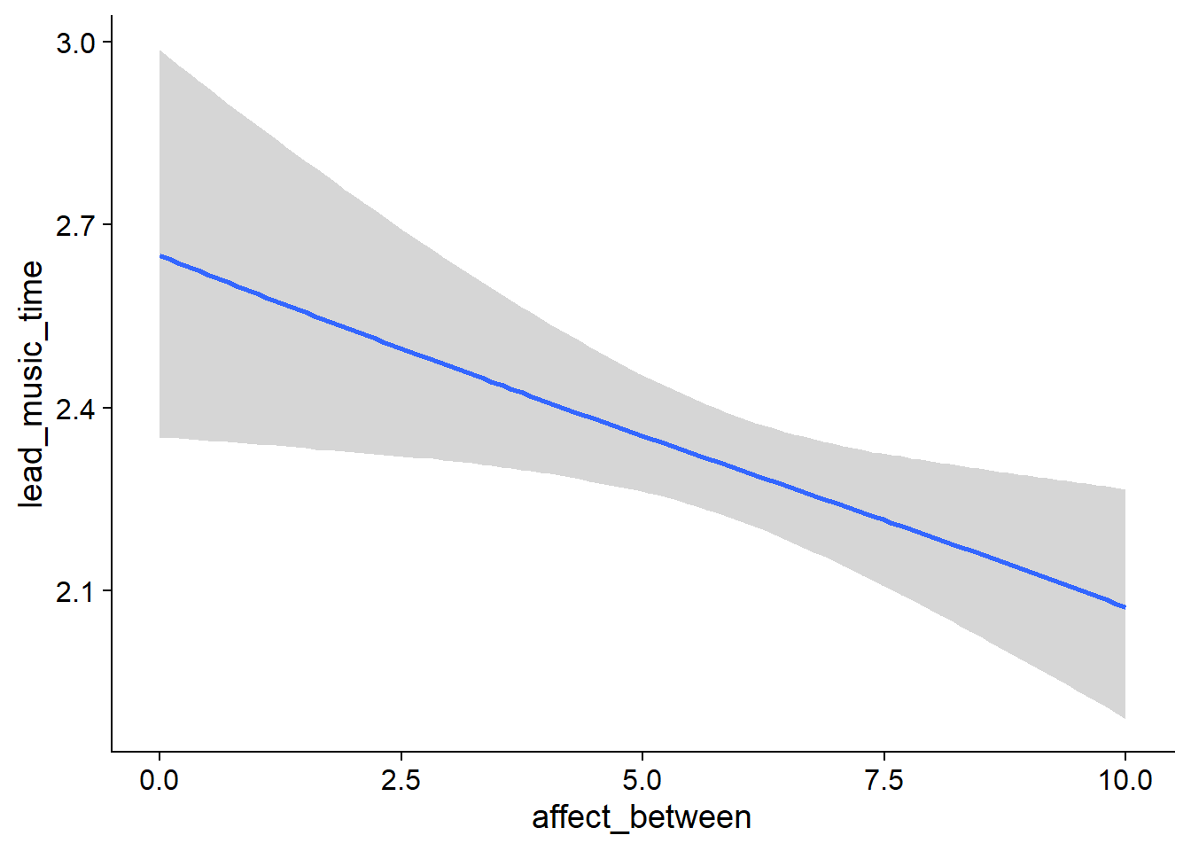
Figure 4.13: Conditional effects for Music-Affect model
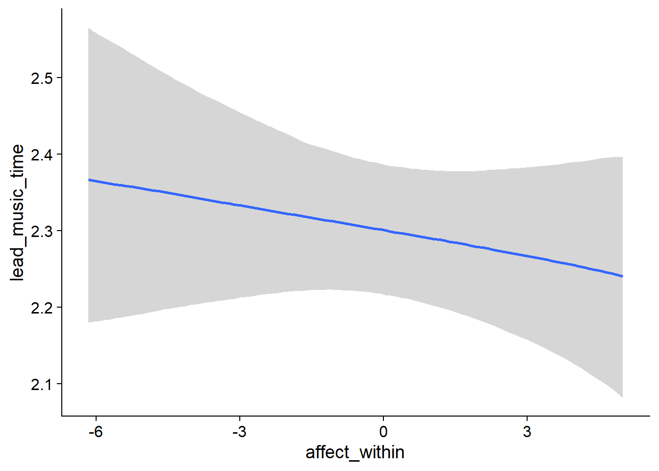
Figure 4.14: Conditional effects for Music-Affect model
##            used  (Mb) gc trigger   (Mb)  max used   (Mb)
## Ncells  3691581 197.2    6044351  322.9   6044351  322.9
## Vcells 23766048 181.4  173752545 1325.7 217189556 1657.1
4.2.2 Life Satisfaction
From now on, I’ll be less verbose in describing the models, simply because we’re running 28 in total (7 categories x two directions x 2 well-being measures). I’ll apply the same steps as I did above with affect and music, but won’t describe every parameter unless there’s something unusual that sticks out. Rather, in the end of this section, I’ll create a summary figure.
4.2.2.1 Music on Life Satisfaction
Let’s run the model. Again, that took about half an hour on my machine.
music_life <-
  brm(
    data = working_file,
    family = gaussian,
    life_satisfaction ~
      1 +
      music_used_between +
      music_used_within +
      music_time_between +
      music_time_within +
      (1 +
         music_time_within +
         music_used_within
       | id),
    iter = 5000,
    warmup = 2000,
    chains = 4,
    cores = 4,
    seed = 42,
    control = list(adapt_delta = 0.95),
    file = here("models", "music_life")
  )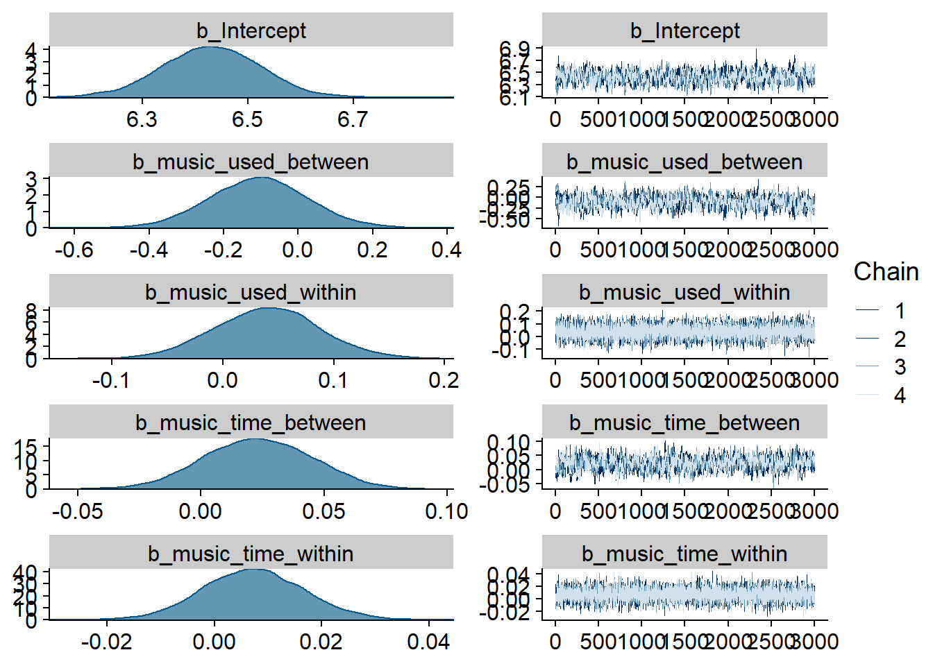
Figure 4.15: Traceplots and posterior distributions for Music-Life Satisfaction model
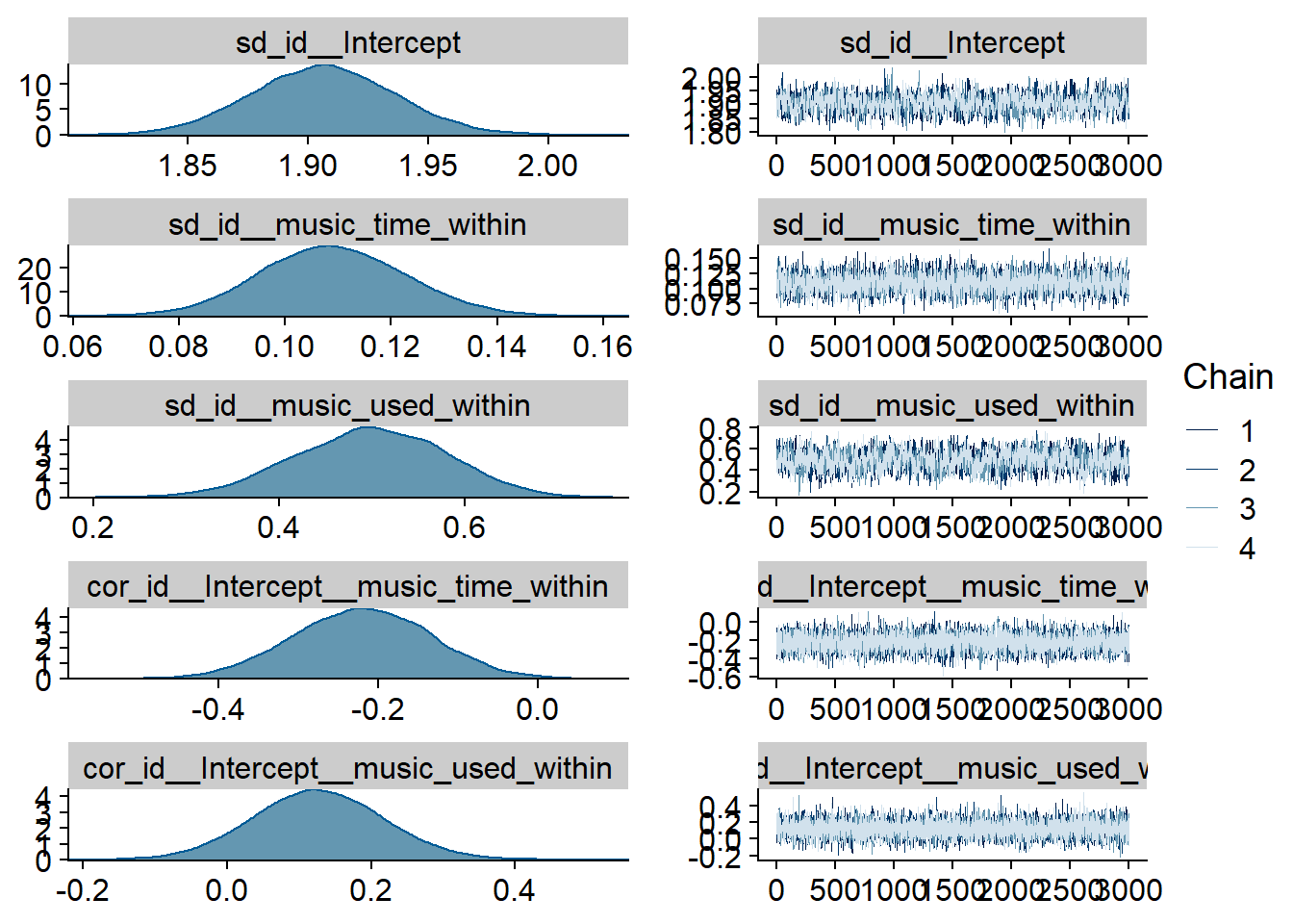
Figure 4.16: Traceplots and posterior distributions for Music-Life Satisfaction model
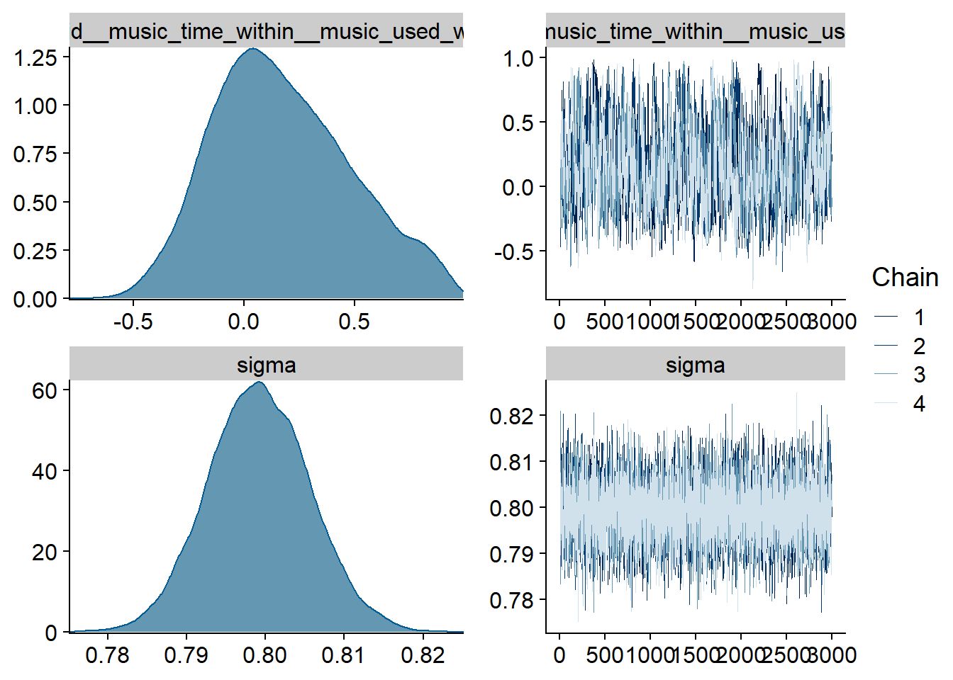
Figure 4.17: Traceplots and posterior distributions for Music-Life Satisfaction model
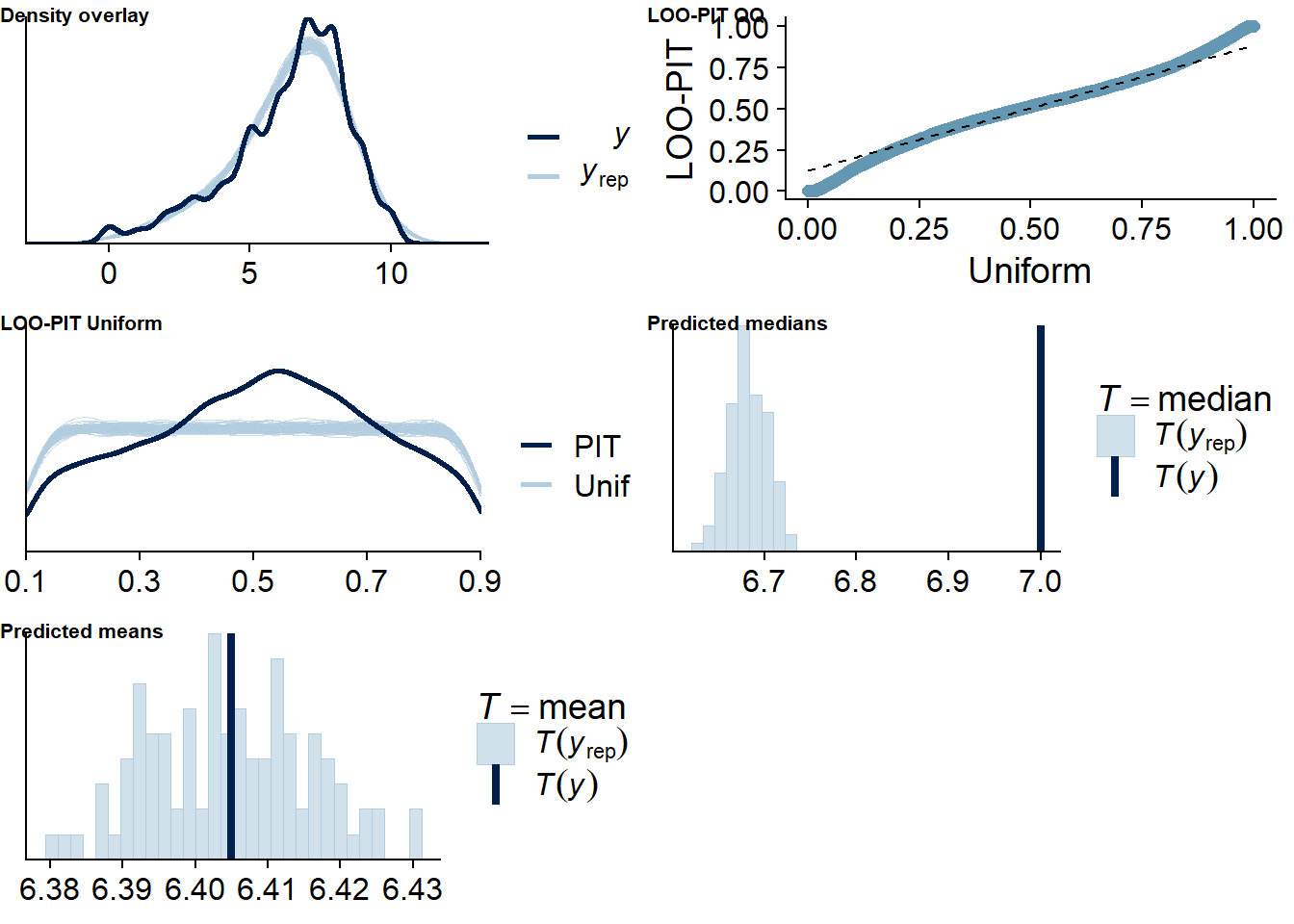
Figure 4.18: Posterior predictive checks for Music-Life Satisfaction model
The outliers are in about the same range as in previous models, and the model diagnostics look good.
music_life_loo <- loo(music_life)
music_life_loo
##
## Computed from 12000 by 10985 log-likelihood matrix
##
## Estimate SE
## elpd_loo -14530.0 147.9
## p_loo 2289.4 54.1
## looic 29059.9 295.8
## ------
## Monte Carlo SE of elpd_loo is NA.
##
## Pareto k diagnostic values:
## Count Pct. Min. n_eff
## (-Inf, 0.5] (good) 10210 92.9% 623
## (0.5, 0.7] (ok) 623 5.7% 101
## (0.7, 1] (bad) 137 1.2% 14
## (1, Inf) (very bad) 15 0.1% 1
## See help('pareto-k-diagnostic') for details.Let’s inspect the summary. We see that:
- Music listeners had lower satisfaction with life than non-listeners (
music_used_between), but the effect is much smaller than for affect and the posterior contains both zero and a lot of negative values - However, if a person went from not listening to listening, they reported higher life satisfaction nthe next week (
music_used_within), but posterior contains zero. - When a person listened to one hour more music than someone else, that person reported slightly higher life satisfaction (
music_time_between), but 0 is in CI. - The same goes for a one-hour increase from one’s typical music listening (
music_time_within): the effect is positive, but super small and the posterior contains zero as well as negative values.
summary(music_life)## Family: gaussian
## Links: mu = identity; sigma = identity
## Formula: life_satisfaction ~ 1 + music_used_between + music_used_within + music_time_between + music_time_within + (1 + music_time_within + music_used_within | id)
## Data: working_file (Number of observations: 10985)
## Samples: 4 chains, each with iter = 5000; warmup = 2000; thin = 1;
## total post-warmup samples = 12000
##
## Group-Level Effects:
## ~id (Number of levels: 2159)
## Estimate Est.Error l-95% CI u-95% CI Rhat Bulk_ESS Tail_ESS
## sd(Intercept) 1.91 0.03 1.85 1.96 1.01 1211 2309
## sd(music_time_within) 0.11 0.01 0.08 0.14 1.00 2961 5824
## sd(music_used_within) 0.50 0.08 0.33 0.65 1.00 818 2361
## cor(Intercept,music_time_within) -0.22 0.09 -0.39 -0.06 1.00 8603 9541
## cor(Intercept,music_used_within) 0.13 0.09 -0.05 0.31 1.00 8745 7147
## cor(music_time_within,music_used_within) 0.18 0.31 -0.36 0.83 1.01 478 752
##
## Population-Level Effects:
## Estimate Est.Error l-95% CI u-95% CI Rhat Bulk_ESS Tail_ESS
## Intercept 6.43 0.09 6.24 6.61 1.01 754 1588
## music_used_between -0.11 0.13 -0.37 0.15 1.01 536 1281
## music_used_within 0.04 0.05 -0.05 0.13 1.00 15623 10202
## music_time_between 0.02 0.02 -0.02 0.07 1.01 819 1615
## music_time_within 0.01 0.01 -0.01 0.03 1.00 11135 9998
##
## Family Specific Parameters:
## Estimate Est.Error l-95% CI u-95% CI Rhat Bulk_ESS Tail_ESS
## sigma 0.80 0.01 0.79 0.81 1.00 8930 9477
##
## Samples were drawn using sampling(NUTS). For each parameter, Bulk_ESS
## and Tail_ESS are effective sample size measures, and Rhat is the potential
## scale reduction factor on split chains (at convergence, Rhat = 1).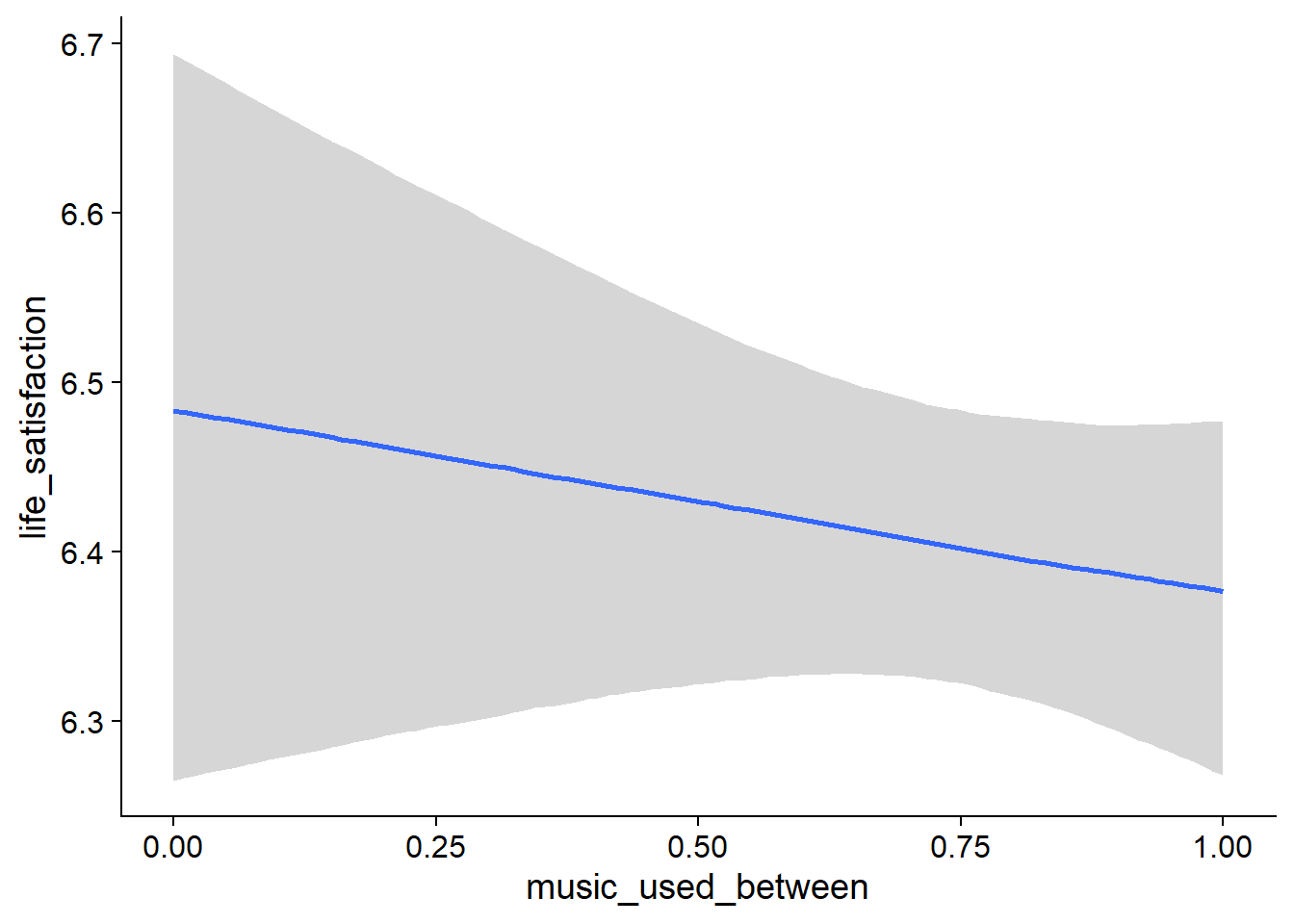
Figure 4.19: Conditional effects for Music-Affect model
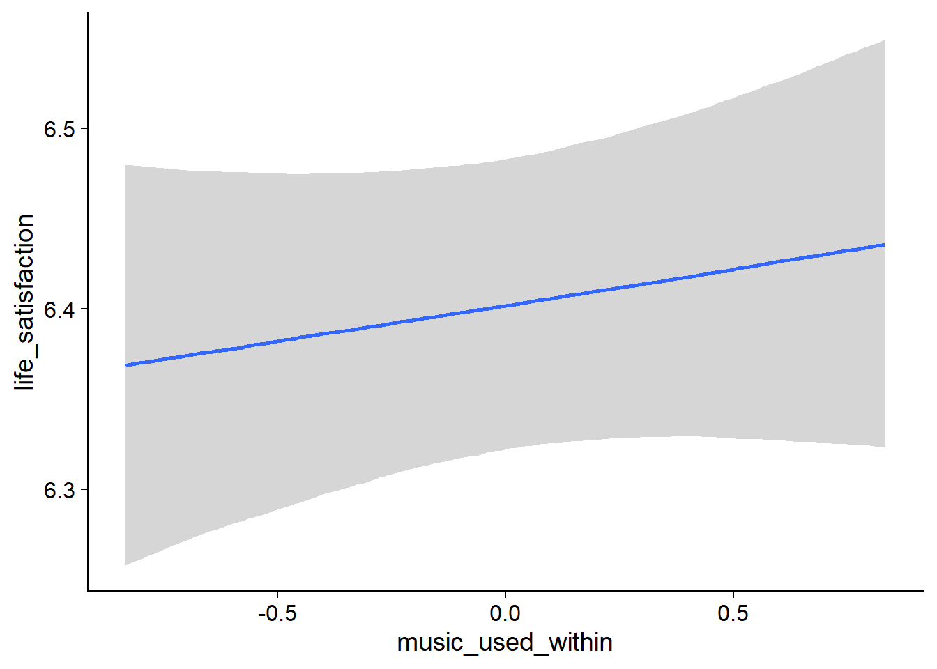
Figure 4.20: Conditional effects for Music-Affect model
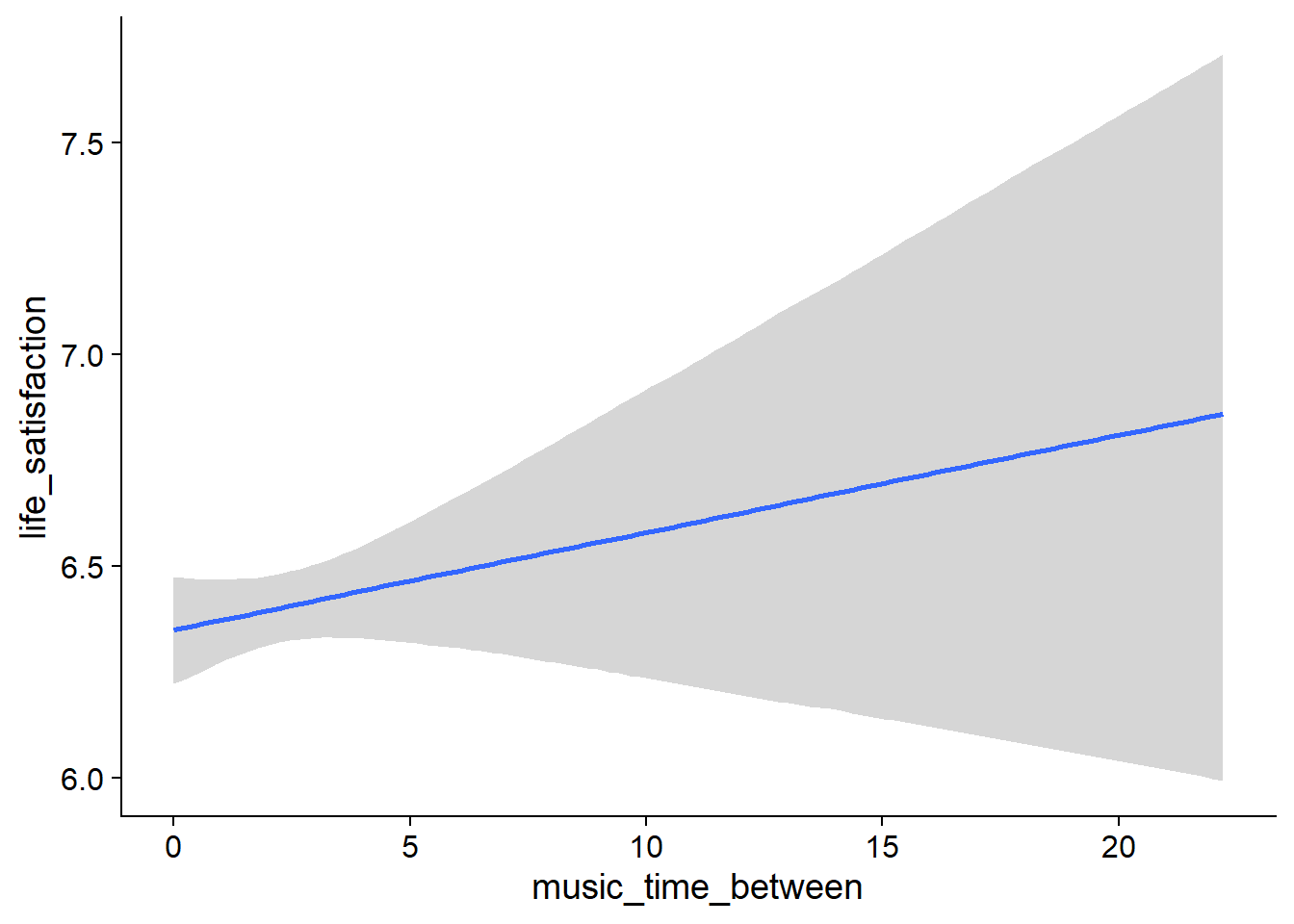
Figure 4.21: Conditional effects for Music-Affect model

Figure 4.22: Conditional effects for Music-Affect model
##            used  (Mb) gc trigger   (Mb)  max used   (Mb)
## Ncells  3691671 197.2    6044351  322.9   6044351  322.9
## Vcells 23766998 181.4  139002036 1060.6 217189556 1657.1
4.2.2.2 Life satisfaction on music
Below I run the model. On my machine, the model took about three and a half hours.
life_music <-
  brm(
    bf(
      # predicting continuous part
      lead_music_time ~
        1 +
        life_satisfaction_between +
        life_satisfaction_within +
        (1 +
           life_satisfaction_within
         | id),

      # predicting hurdle part
      hu ~
        1 +
        life_satisfaction_between +
        life_satisfaction_within +
        (1 +
           life_satisfaction_within
         | id)
    ),
    data = working_file,
    family = hurdle_gamma(),
    ,
    iter = 5000,
    warmup = 2000,
    chains = 4,
    cores = 4,
    seed = 42,
    control = list(adapt_delta = 0.95),
    file = here("models", "life_music")
  )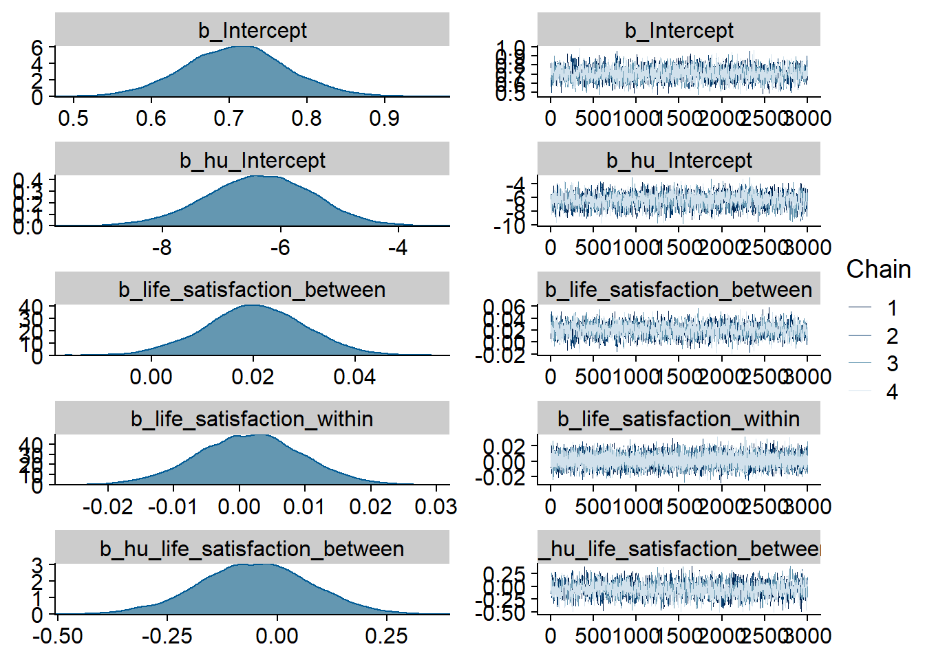
Figure 4.23: Traceplots and posterior distributions for Life Satisfaction-Music model
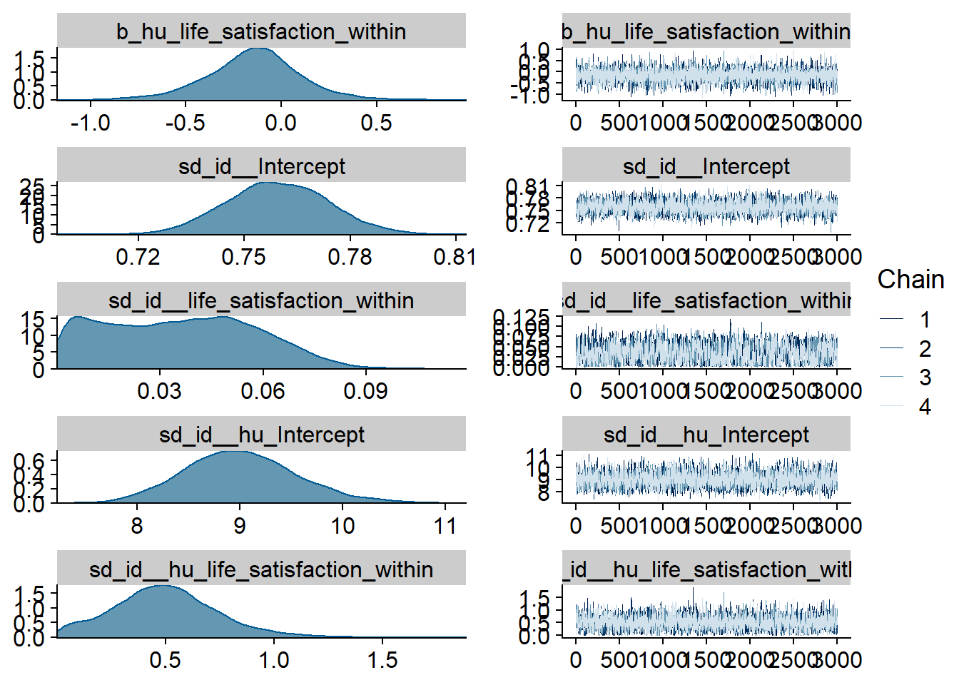
Figure 4.24: Traceplots and posterior distributions for Life Satisfaction-Music model
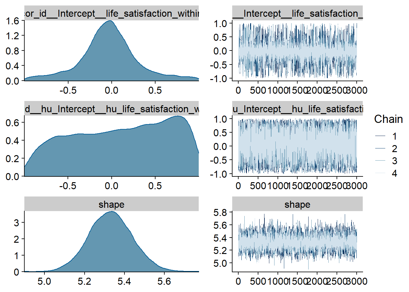
Figure 4.25: Traceplots and posterior distributions for Life Satisfaction-Music model
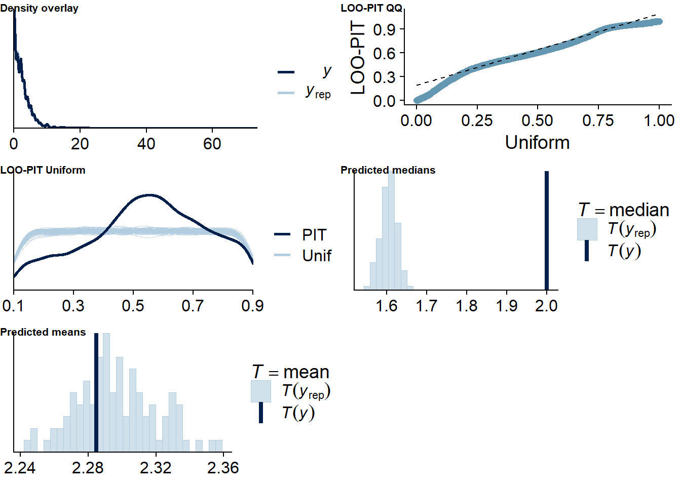
Figure 4.26: Posterior predictive checks for Life Satisfaction-Music model
Once more, there are several potential outliers. Again, because the model diagnostics look good and leaving one out here will estimate parameters for a participant with only two observations, which can lead to influential values, I believe the model is just flexible.
life_music_loo <- loo(life_music)
life_music_loo
##
## Computed from 12000 by 8698 log-likelihood matrix
##
## Estimate SE
## elpd_loo -11513.5 123.2
## p_loo 2082.9 52.6
## looic 23026.9 246.5
## ------
## Monte Carlo SE of elpd_loo is NA.
##
## Pareto k diagnostic values:
## Count Pct. Min. n_eff
## (-Inf, 0.5] (good) 7652 88.0% 701
## (0.5, 0.7] (ok) 676 7.8% 157
## (0.7, 1] (bad) 276 3.2% 10
## (1, Inf) (very bad) 94 1.1% 1
## See help('pareto-k-diagnostic') for details.Summary:
- Those with higher life satisfaction have a (very small) tendency to listen to more music a week later than those with lower life satisfaction:
exp(0.02)= 1.02 (life_satisfaction_between) - As a person goes up one point on affect compared to their typical life satisfaction score, their music time increases by a factor of
exp(0.002)= 1 - a completely negligible, small effect whose posterior includes zero (life_satisfaction_within). - The between effect shows that people with higher life satisfaction also have lower odds of not listening to music across all waves:
exp(-0.31)= 0.733447 forhu_life_satisfaction_between- but the posterior goes from negative to positive. - If the average users went went up one point from their typical life satisfaction score, they had lower odds of not listening to music a week later,
exp(-0.15)= 0.860708, but again the posterior includes a wide range of values, including zero.
summary(life_music)## Family: hurdle_gamma
## Links: mu = log; shape = identity; hu = logit
## Formula: lead_music_time ~ 1 + life_satisfaction_between + life_satisfaction_within + (1 + life_satisfaction_within | id)
## hu ~ 1 + life_satisfaction_between + life_satisfaction_within + (1 + life_satisfaction_within | id)
## Data: working_file (Number of observations: 8698)
## Samples: 4 chains, each with iter = 5000; warmup = 2000; thin = 1;
## total post-warmup samples = 12000
##
## Group-Level Effects:
## ~id (Number of levels: 2157)
## Estimate Est.Error l-95% CI u-95% CI Rhat Bulk_ESS Tail_ESS
## sd(Intercept) 0.76 0.01 0.73 0.79 1.00 2364 4922
## sd(life_satisfaction_within) 0.04 0.02 0.00 0.08 1.00 1295 3789
## sd(hu_Intercept) 9.01 0.55 8.00 10.19 1.00 3125 5342
## sd(hu_life_satisfaction_within) 0.50 0.24 0.06 1.02 1.00 2794 3283
## cor(Intercept,life_satisfaction_within) -0.03 0.34 -0.78 0.75 1.00 9234 4000
## cor(hu_Intercept,hu_life_satisfaction_within) 0.11 0.55 -0.88 0.94 1.00 5983 6577
##
## Population-Level Effects:
## Estimate Est.Error l-95% CI u-95% CI Rhat Bulk_ESS Tail_ESS
## Intercept 0.71 0.07 0.58 0.84 1.00 1752 3009
## hu_Intercept -6.36 0.90 -8.17 -4.64 1.00 1794 3694
## life_satisfaction_between 0.02 0.01 0.00 0.04 1.00 1669 3526
## life_satisfaction_within 0.00 0.01 -0.01 0.02 1.00 16724 9671
## hu_life_satisfaction_between -0.05 0.13 -0.31 0.19 1.00 1651 3214
## hu_life_satisfaction_within -0.15 0.25 -0.68 0.36 1.00 6065 7309
##
## Family Specific Parameters:
## Estimate Est.Error l-95% CI u-95% CI Rhat Bulk_ESS Tail_ESS
## shape 5.33 0.11 5.12 5.55 1.00 6693 8054
##
## Samples were drawn using sampling(NUTS). For each parameter, Bulk_ESS
## and Tail_ESS are effective sample size measures, and Rhat is the potential
## scale reduction factor on split chains (at convergence, Rhat = 1).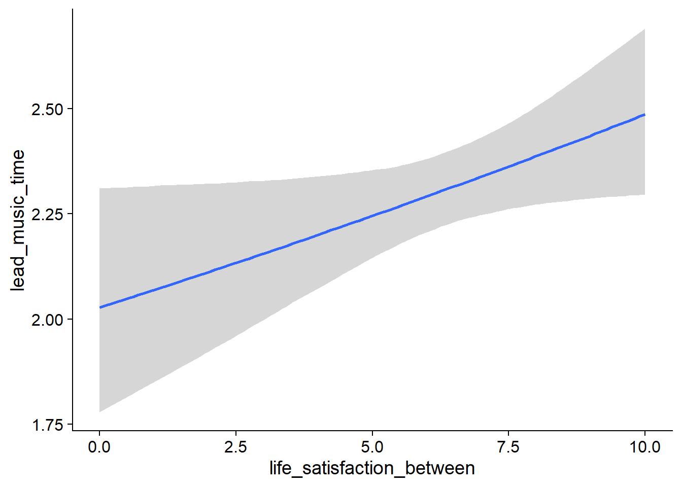
Figure 4.27: Conditional effects for Life Satisfaction-Music model
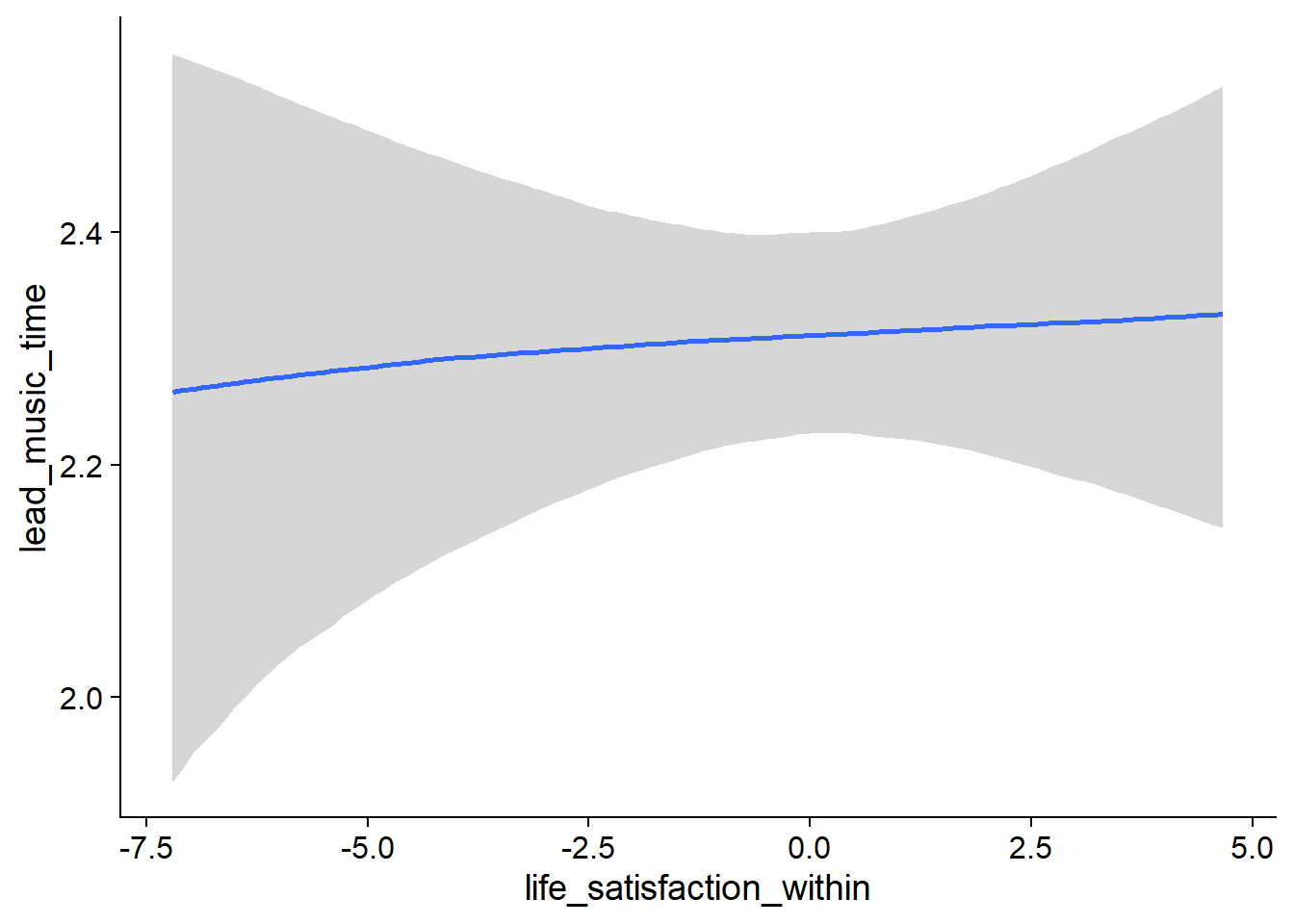
Figure 4.28: Conditional effects for Life Satisfaction-Music model
##            used  (Mb) gc trigger   (Mb)  max used   (Mb)
## Ncells  3691793 197.2    6044351  322.9   6044351  322.9
## Vcells 23768137 181.4  196642498 1500.3 217189556 1657.1
4.3 Films
4.3.1 Affect
4.3.1.1 Films on affect
films_affect <-
  brm(
    data = working_file,
    family = gaussian,
    affect ~
      1 +
      films_used_between +
      films_used_within +
      films_time_between +
      films_time_within +
      (1 +
         films_time_within +
         films_used_within
       | id),
    iter = 5000,
    warmup = 2000,
    chains = 4,
    cores = 4,
    seed = 42,
    control = list(adapt_delta = 0.95),
    file = here("models", "films_affect")
  )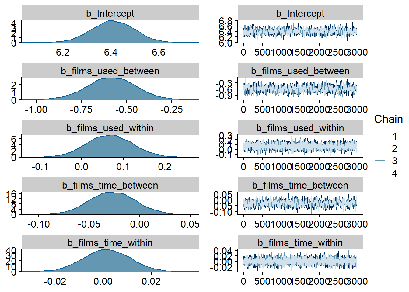
Figure 4.29: Traceplots and posterior distributions for Films-Affect model
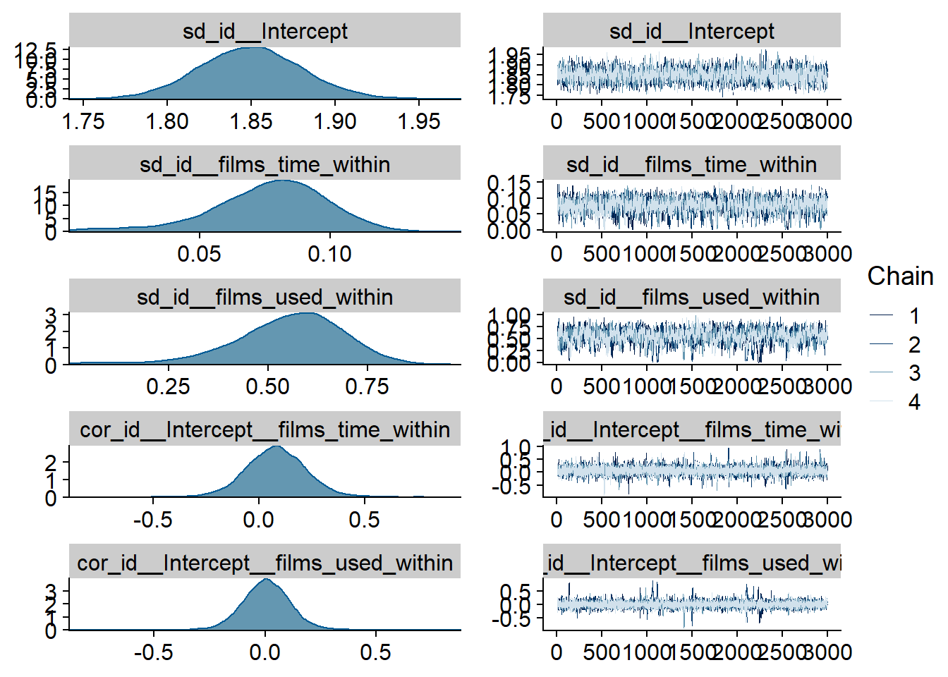
Figure 4.30: Traceplots and posterior distributions for Films-Affect model
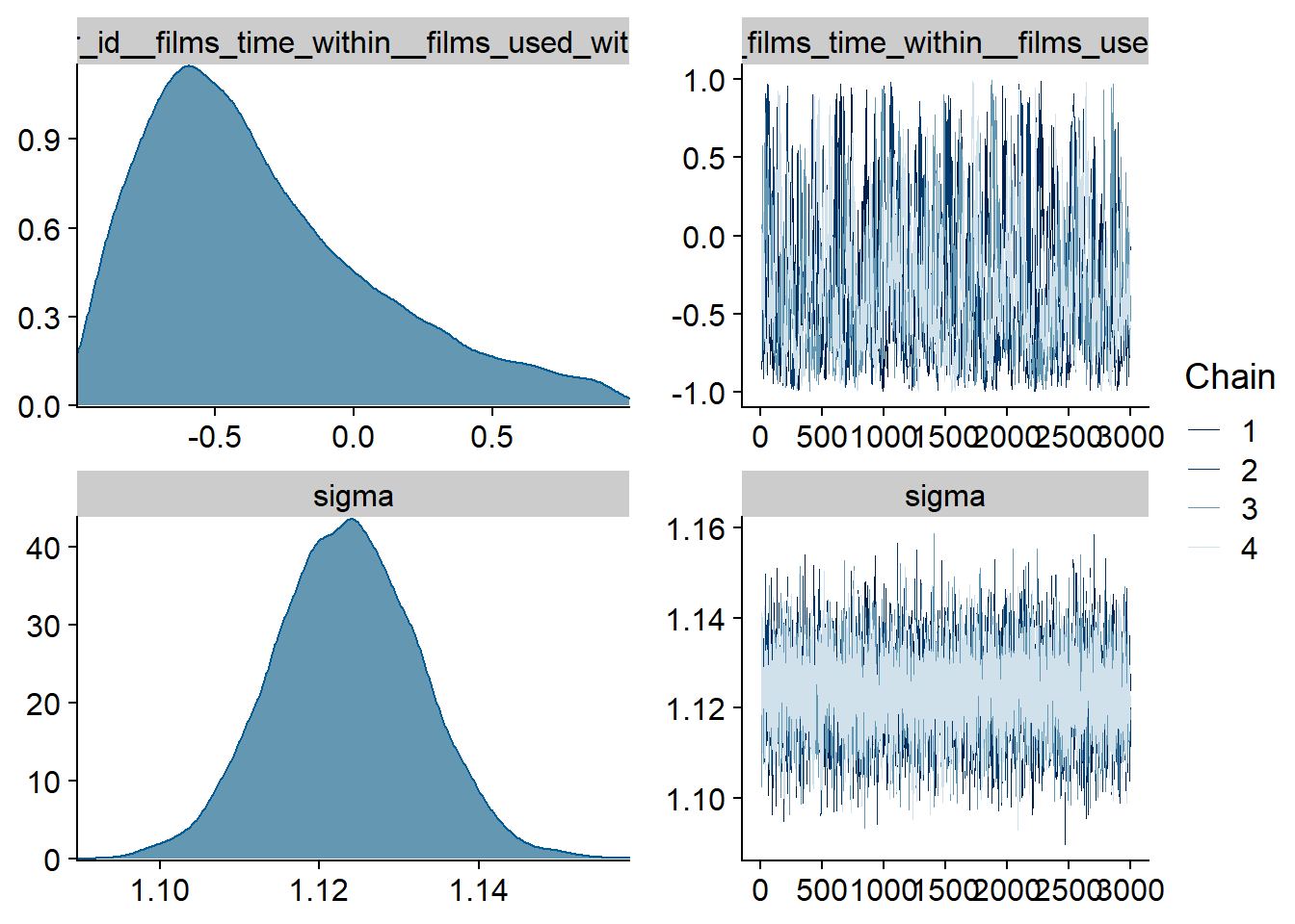
Figure 4.31: Traceplots and posterior distributions for Films-Affect model
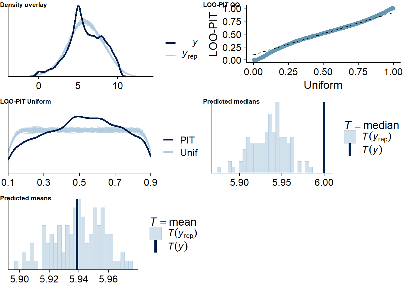
Figure 4.32: Posterior predictive checks for Films-Affect model
The outliers are in about the same range as in previous models, and the model diagnostics look good.
films_affect_loo <- loo(films_affect)
films_affect_loo
##
## Computed from 12000 by 10985 log-likelihood matrix
##
## Estimate SE
## elpd_loo -18109.0 105.7
## p_loo 2070.9 36.3
## looic 36218.0 211.4
## ------
## Monte Carlo SE of elpd_loo is NA.
##
## Pareto k diagnostic values:
## Count Pct. Min. n_eff
## (-Inf, 0.5] (good) 10483 95.4% 448
## (0.5, 0.7] (ok) 447 4.1% 152
## (0.7, 1] (bad) 51 0.5% 38
## (1, Inf) (very bad) 4 0.0% 7
## See help('pareto-k-diagnostic') for details.Below the summary.
summary(films_affect)## Family: gaussian
## Links: mu = identity; sigma = identity
## Formula: affect ~ 1 + films_used_between + films_used_within + films_time_between + films_time_within + (1 + films_time_within + films_used_within | id)
## Data: working_file (Number of observations: 10985)
## Samples: 4 chains, each with iter = 5000; warmup = 2000; thin = 1;
## total post-warmup samples = 12000
##
## Group-Level Effects:
## ~id (Number of levels: 2159)
## Estimate Est.Error l-95% CI u-95% CI Rhat Bulk_ESS Tail_ESS
## sd(Intercept) 1.85 0.03 1.79 1.91 1.00 2468 4159
## sd(films_time_within) 0.08 0.02 0.02 0.12 1.00 1657 1479
## sd(films_used_within) 0.55 0.14 0.22 0.79 1.00 768 785
## cor(Intercept,films_time_within) 0.08 0.16 -0.22 0.39 1.00 7871 4187
## cor(Intercept,films_used_within) 0.01 0.12 -0.21 0.23 1.00 8904 4186
## cor(films_time_within,films_used_within) -0.34 0.42 -0.92 0.69 1.00 522 1078
##
## Population-Level Effects:
## Estimate Est.Error l-95% CI u-95% CI Rhat Bulk_ESS Tail_ESS
## Intercept 6.41 0.09 6.23 6.58 1.00 1658 3026
## films_used_between -0.58 0.14 -0.85 -0.31 1.00 1523 2729
## films_used_within 0.07 0.06 -0.04 0.18 1.00 18132 10024
## films_time_between -0.03 0.02 -0.07 0.02 1.00 1795 3445
## films_time_within 0.00 0.01 -0.02 0.02 1.00 15647 10134
##
## Family Specific Parameters:
## Estimate Est.Error l-95% CI u-95% CI Rhat Bulk_ESS Tail_ESS
## sigma 1.12 0.01 1.11 1.14 1.00 6560 8297
##
## Samples were drawn using sampling(NUTS). For each parameter, Bulk_ESS
## and Tail_ESS are effective sample size measures, and Rhat is the potential
## scale reduction factor on split chains (at convergence, Rhat = 1).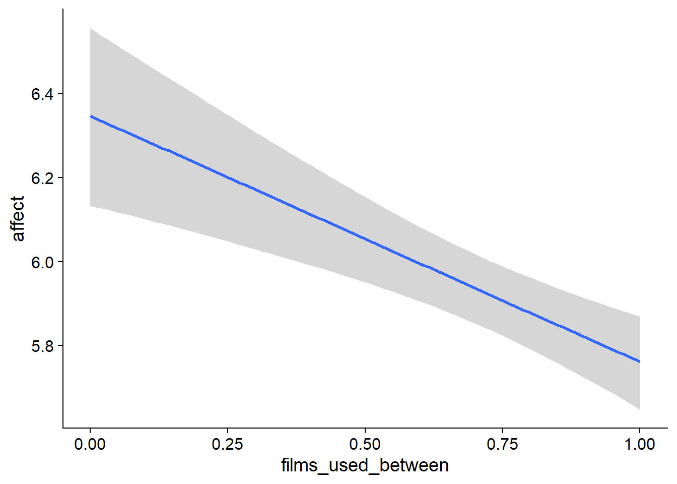
Figure 4.33: Conditional effects for Films-Affect model
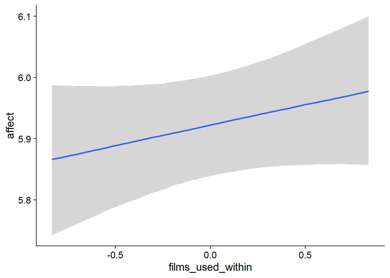
Figure 4.34: Conditional effects for Films-Affect model
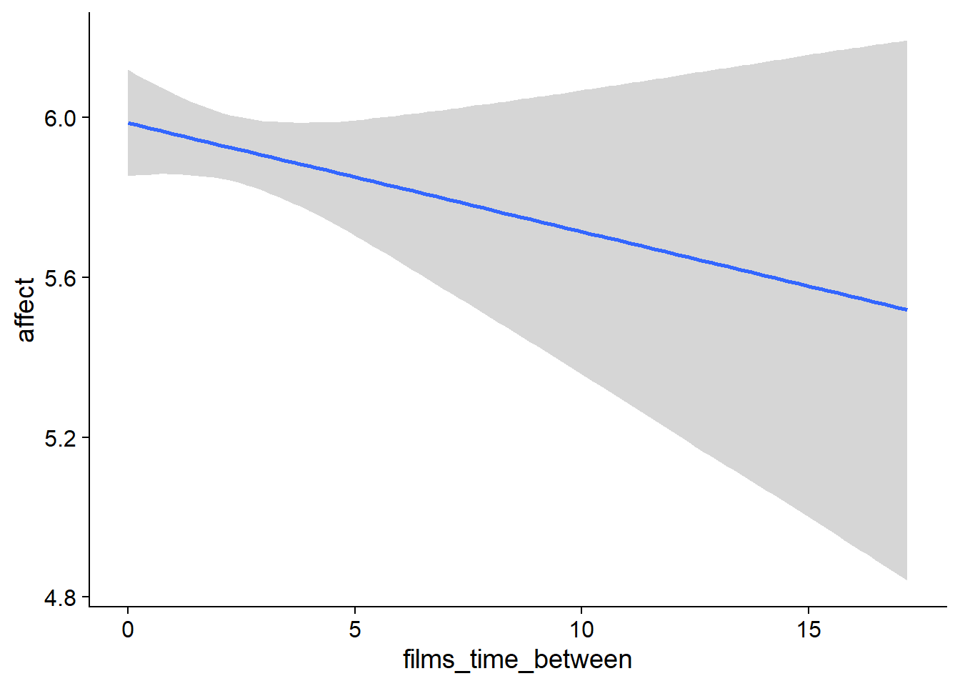
Figure 4.35: Conditional effects for Films-Affect model
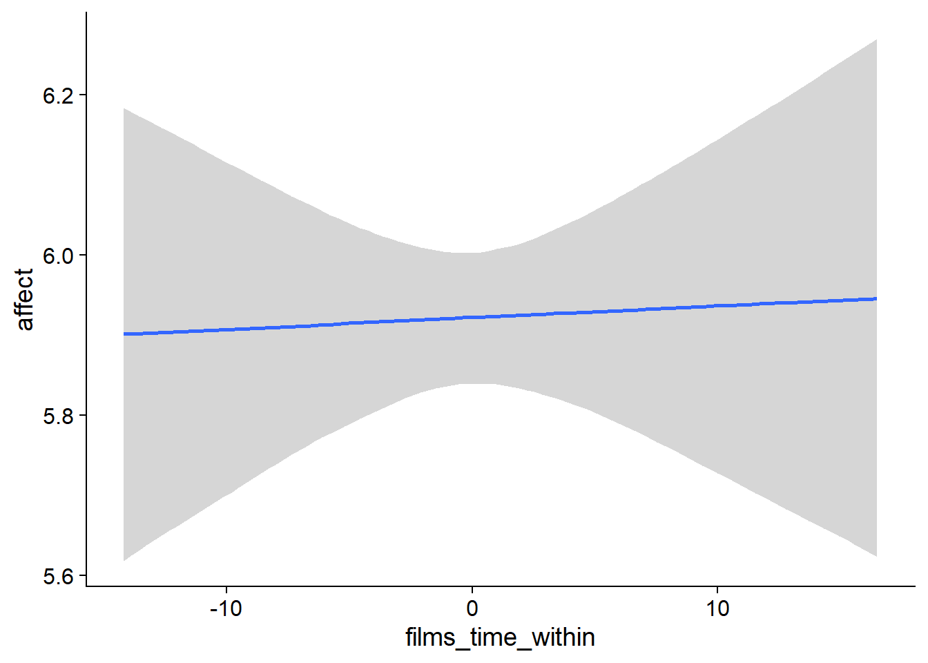
Figure 4.36: Conditional effects for Films-Affect model
##            used  (Mb) gc trigger   (Mb)  max used   (Mb)
## Ncells  3691953 197.2    6044351  322.9   6044351  322.9
## Vcells 23769215 181.4  157313999 1200.3 217189556 1657.1
4.3.1.2 Affect on films
affect_films <-
  brm(
    bf(
      # predicting continuous part
      lead_films_time ~
        1 +
        affect_between +
        affect_within +
        (1 +
           affect_within
         | id),

      # predicting hurdle part
      hu ~
        1 +
        affect_between +
        affect_within +
        (1 +
           affect_within
         | id)
    ),
    data = working_file,
    family = hurdle_gamma(),
    ,
    iter = 5000,
    warmup = 2000,
    chains = 4,
    cores = 4,
    seed = 42,
    control = list(adapt_delta = 0.95),
    file = here("models", "affect_films")
  )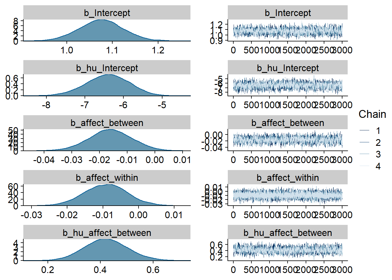
Figure 4.37: Traceplots and posterior distributions for Affect-Films model
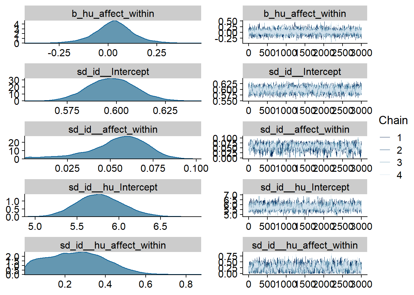
Figure 4.38: Traceplots and posterior distributions for Affect-Films model
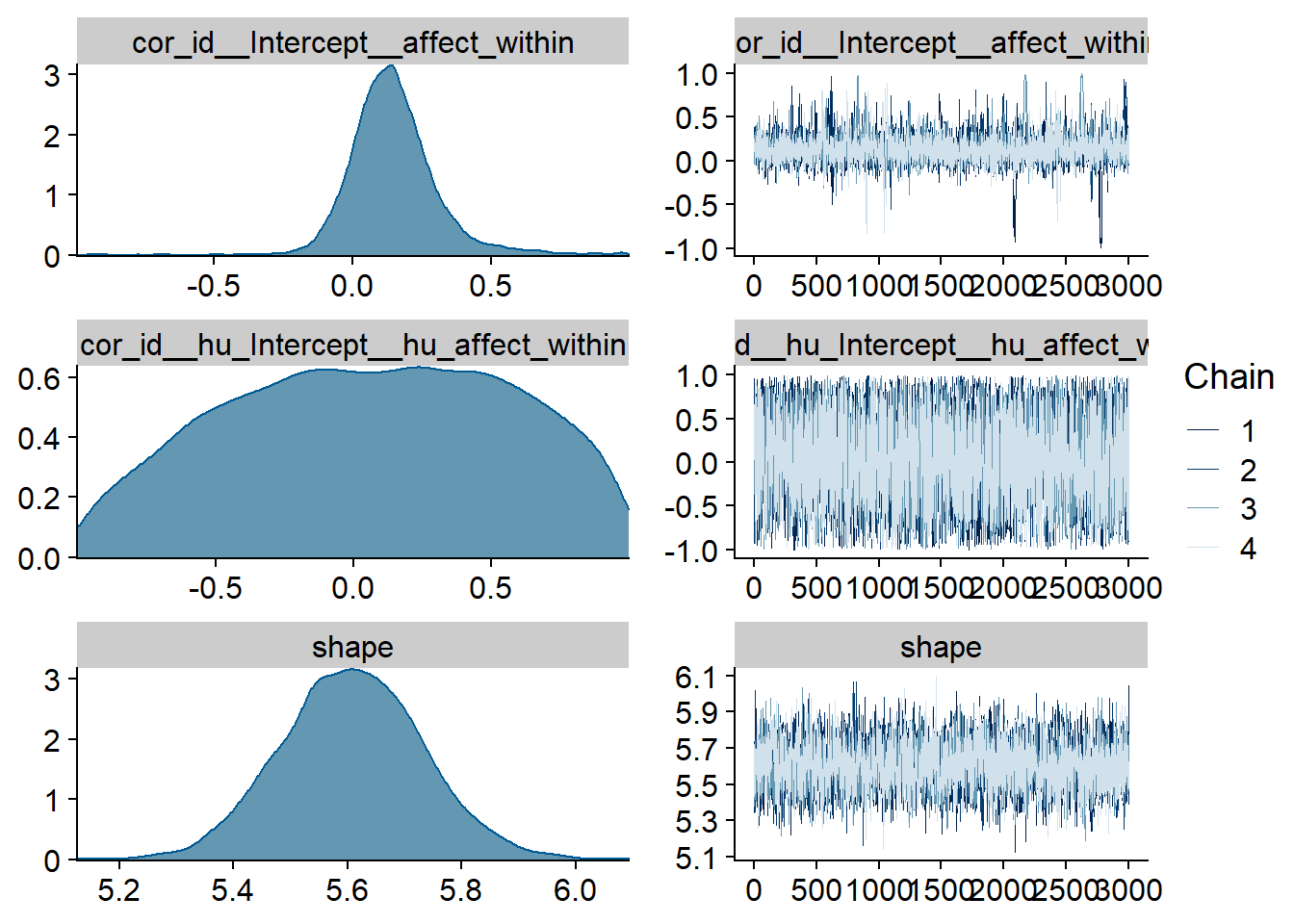
Figure 4.39: Traceplots and posterior distributions for Affect-Films model
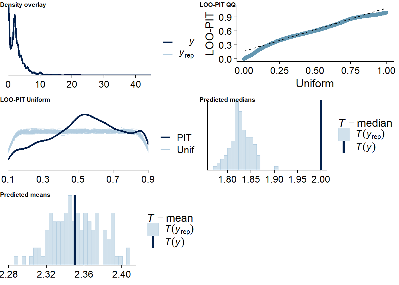
Figure 4.40: Posterior predictive checks for Affect-Films model
The outliers are in about the same range as in previous models, and the model diagnostics look good.
affect_films_loo <- loo(affect_films)
affect_films_loo
##
## Computed from 12000 by 8698 log-likelihood matrix
##
## Estimate SE
## elpd_loo -12653.3 129.0
## p_loo 2333.3 51.9
## looic 25306.6 258.0
## ------
## Monte Carlo SE of elpd_loo is NA.
##
## Pareto k diagnostic values:
## Count Pct. Min. n_eff
## (-Inf, 0.5] (good) 7548 86.8% 546
## (0.5, 0.7] (ok) 689 7.9% 174
## (0.7, 1] (bad) 391 4.5% 12
## (1, Inf) (very bad) 70 0.8% 2
## See help('pareto-k-diagnostic') for details.Below the summary.
summary(affect_films)## Family: hurdle_gamma
## Links: mu = log; shape = identity; hu = logit
## Formula: lead_films_time ~ 1 + affect_between + affect_within + (1 + affect_within | id)
## hu ~ 1 + affect_between + affect_within + (1 + affect_within | id)
## Data: working_file (Number of observations: 8698)
## Samples: 4 chains, each with iter = 5000; warmup = 2000; thin = 1;
## total post-warmup samples = 12000
##
## Group-Level Effects:
## ~id (Number of levels: 2157)
## Estimate Est.Error l-95% CI u-95% CI Rhat Bulk_ESS Tail_ESS
## sd(Intercept) 0.60 0.01 0.57 0.62 1.00 2609 5177
## sd(affect_within) 0.05 0.02 0.01 0.08 1.00 914 708
## sd(hu_Intercept) 5.78 0.28 5.26 6.35 1.00 2593 5498
## sd(hu_affect_within) 0.25 0.14 0.01 0.54 1.00 1062 2592
## cor(Intercept,affect_within) 0.15 0.17 -0.12 0.53 1.00 2342 1348
## cor(hu_Intercept,hu_affect_within) 0.06 0.50 -0.88 0.92 1.00 5887 5689
##
## Population-Level Effects:
## Estimate Est.Error l-95% CI u-95% CI Rhat Bulk_ESS Tail_ESS
## Intercept 1.08 0.05 0.98 1.17 1.00 1812 3613
## hu_Intercept -6.42 0.56 -7.57 -5.36 1.00 1962 3865
## affect_between -0.02 0.01 -0.03 -0.00 1.00 1849 3035
## affect_within -0.01 0.01 -0.02 0.00 1.00 14139 10391
## hu_affect_between 0.42 0.08 0.26 0.59 1.00 1952 3896
## hu_affect_within 0.03 0.10 -0.18 0.23 1.00 5926 6769
##
## Family Specific Parameters:
## Estimate Est.Error l-95% CI u-95% CI Rhat Bulk_ESS Tail_ESS
## shape 5.61 0.12 5.37 5.85 1.00 3085 6328
##
## Samples were drawn using sampling(NUTS). For each parameter, Bulk_ESS
## and Tail_ESS are effective sample size measures, and Rhat is the potential
## scale reduction factor on split chains (at convergence, Rhat = 1).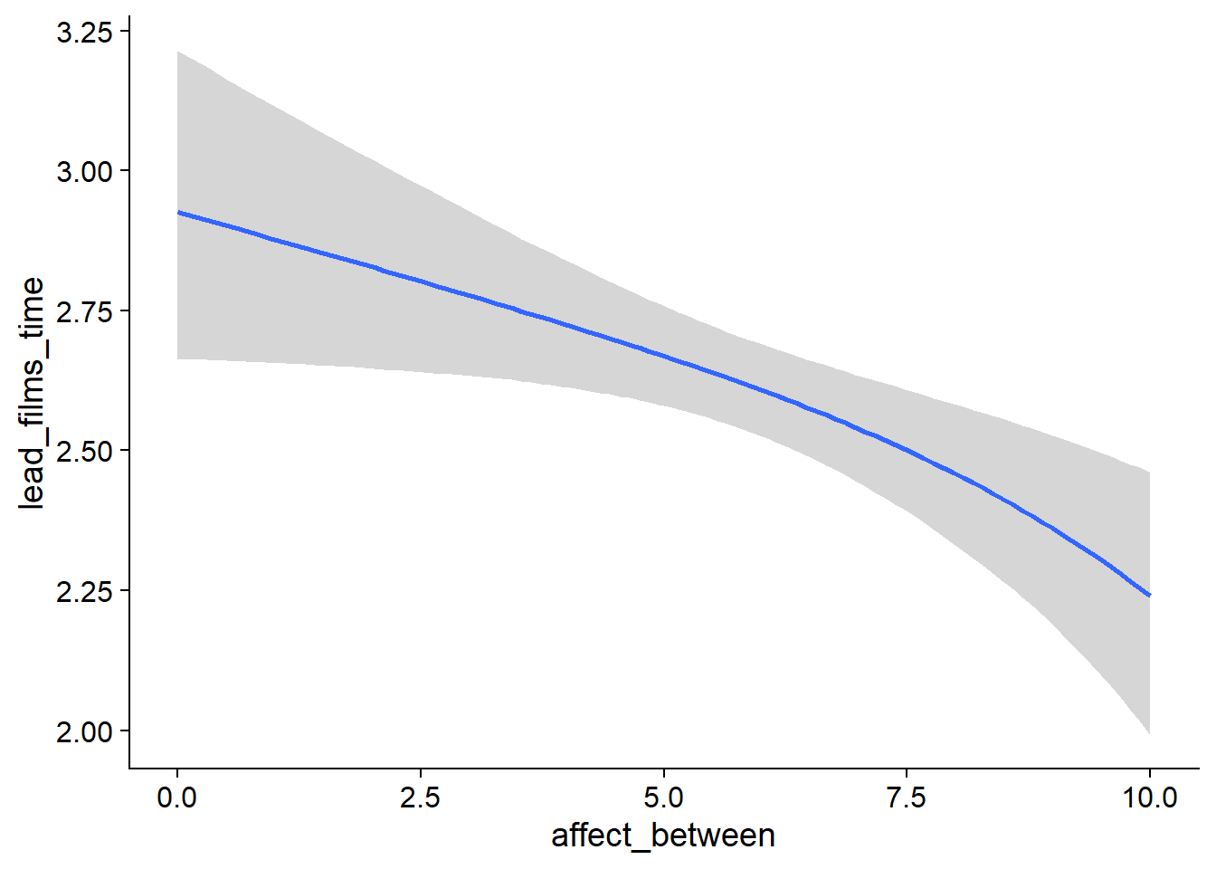
Figure 4.41: Conditional effects for Affect-Films model
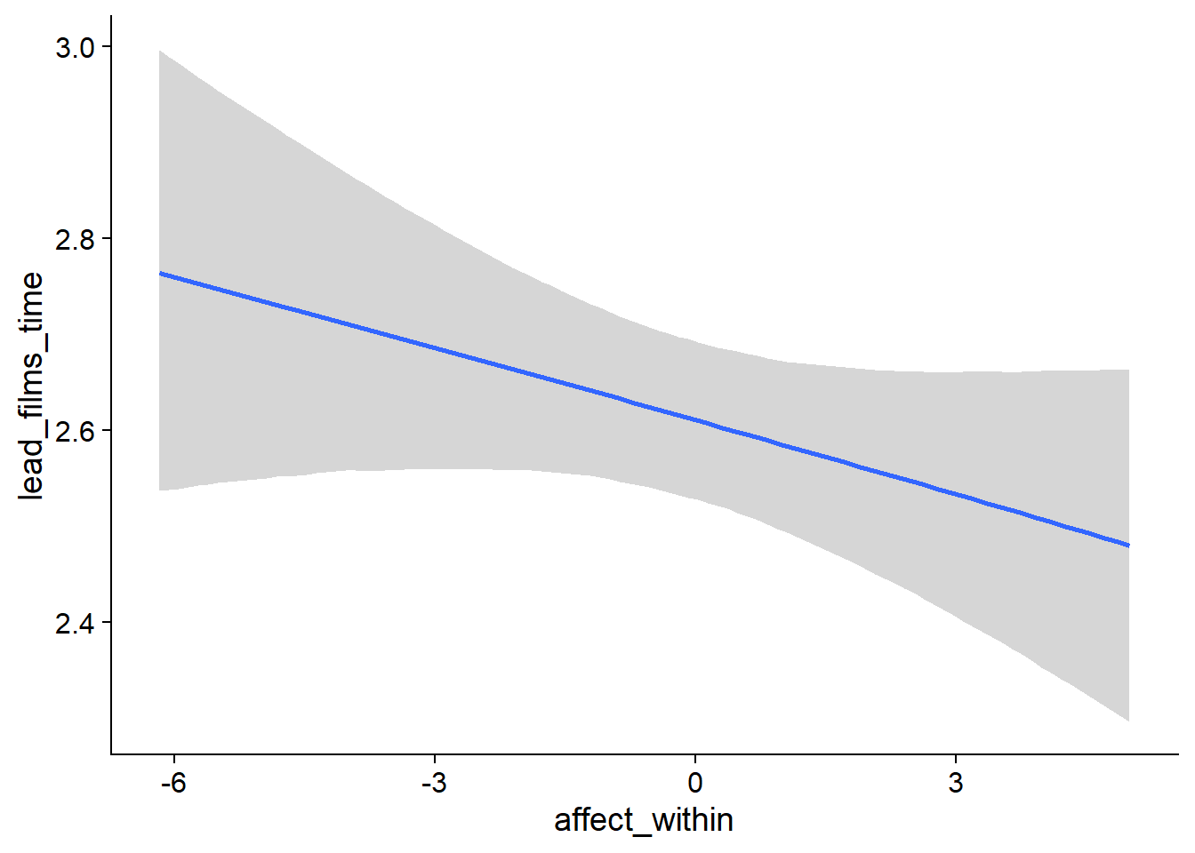
Figure 4.42: Conditional effects for Affect-Films model
##            used  (Mb) gc trigger   (Mb)  max used   (Mb)
## Ncells  3692050 197.2    6044351  322.9   6044351  322.9
## Vcells 23770143 181.4  184915906 1410.8 221148237 1687.3
4.3.2 Life satisfaction
4.3.2.1 Films on life satisfaction
films_life <-
  brm(
    data = working_file,
    family = gaussian,
    life_satisfaction ~
      1 +
      films_used_between +
      films_used_within +
      films_time_between +
      films_time_within +
      (1 +
         films_time_within +
         films_used_within
       | id),
    iter = 5000,
    warmup = 2000,
    chains = 4,
    cores = 4,
    seed = 42,
    control = list(adapt_delta = 0.95),
    file = here("models", "films_life")
  )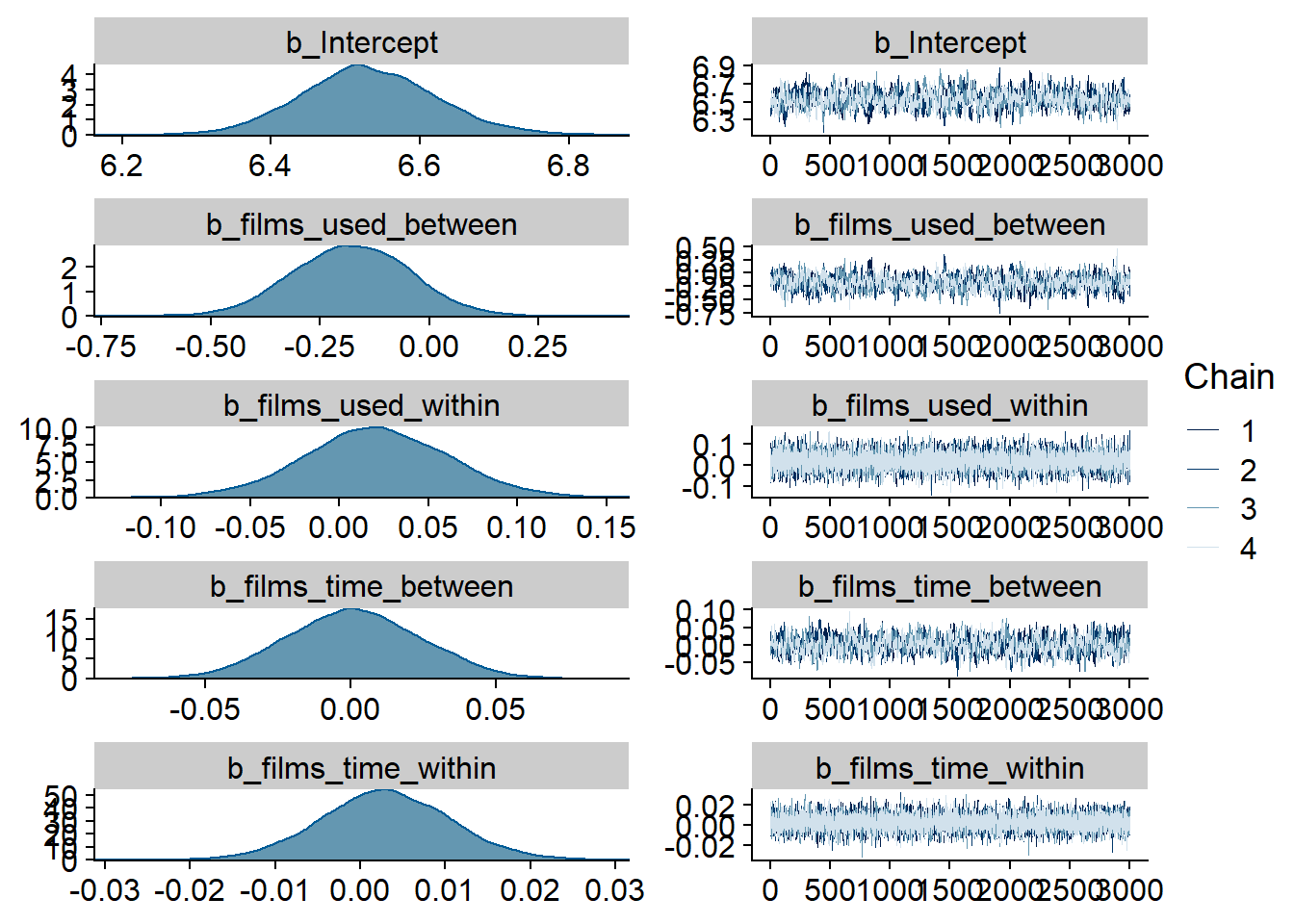
Figure 4.43: Traceplots and posterior distributions for Films-Life Satisfaction model
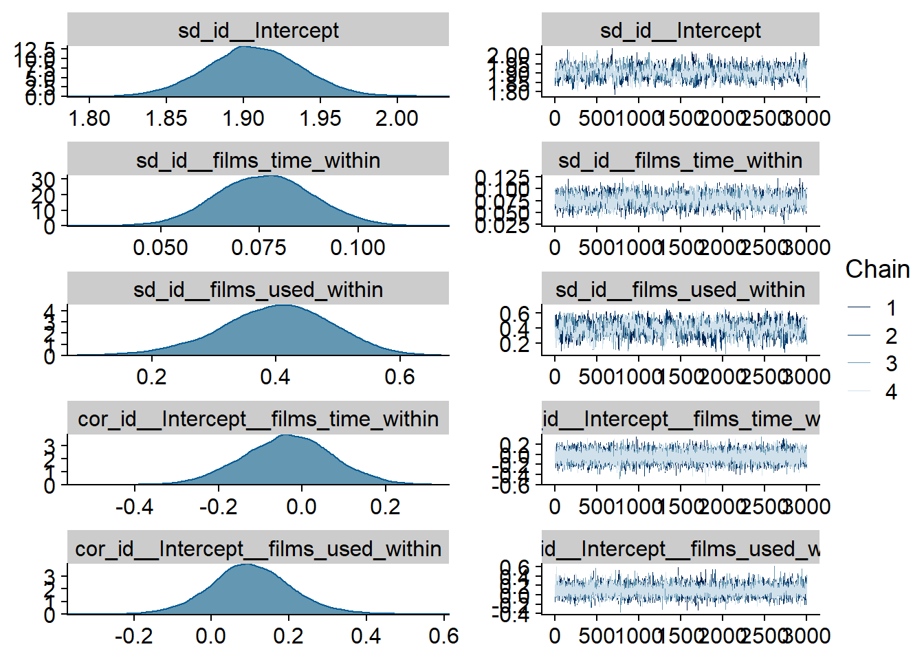
Figure 4.44: Traceplots and posterior distributions for Films-Life Satisfaction model
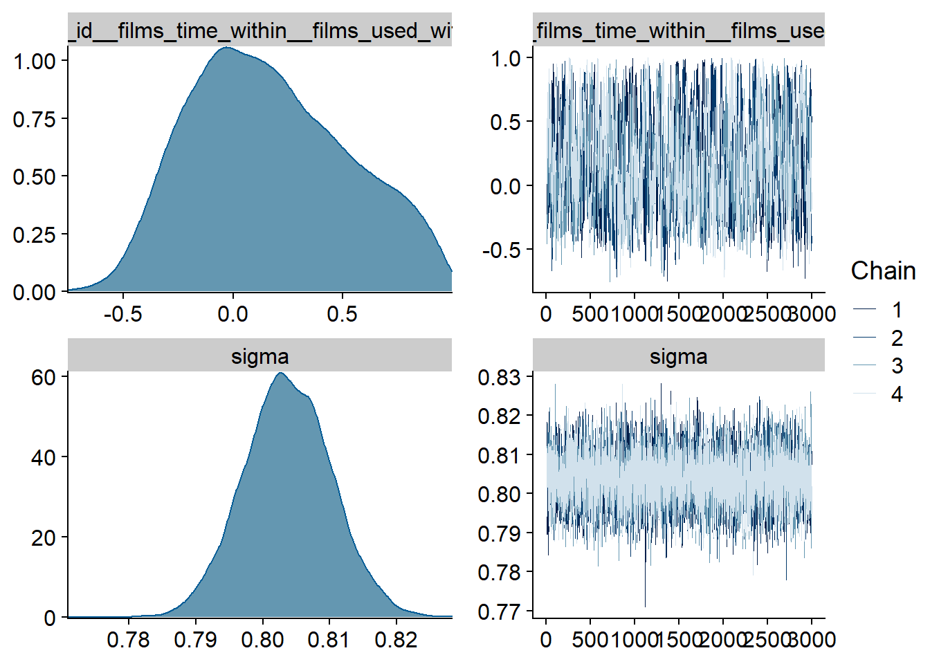
Figure 4.45: Traceplots and posterior distributions for Films-Life Satisfaction model
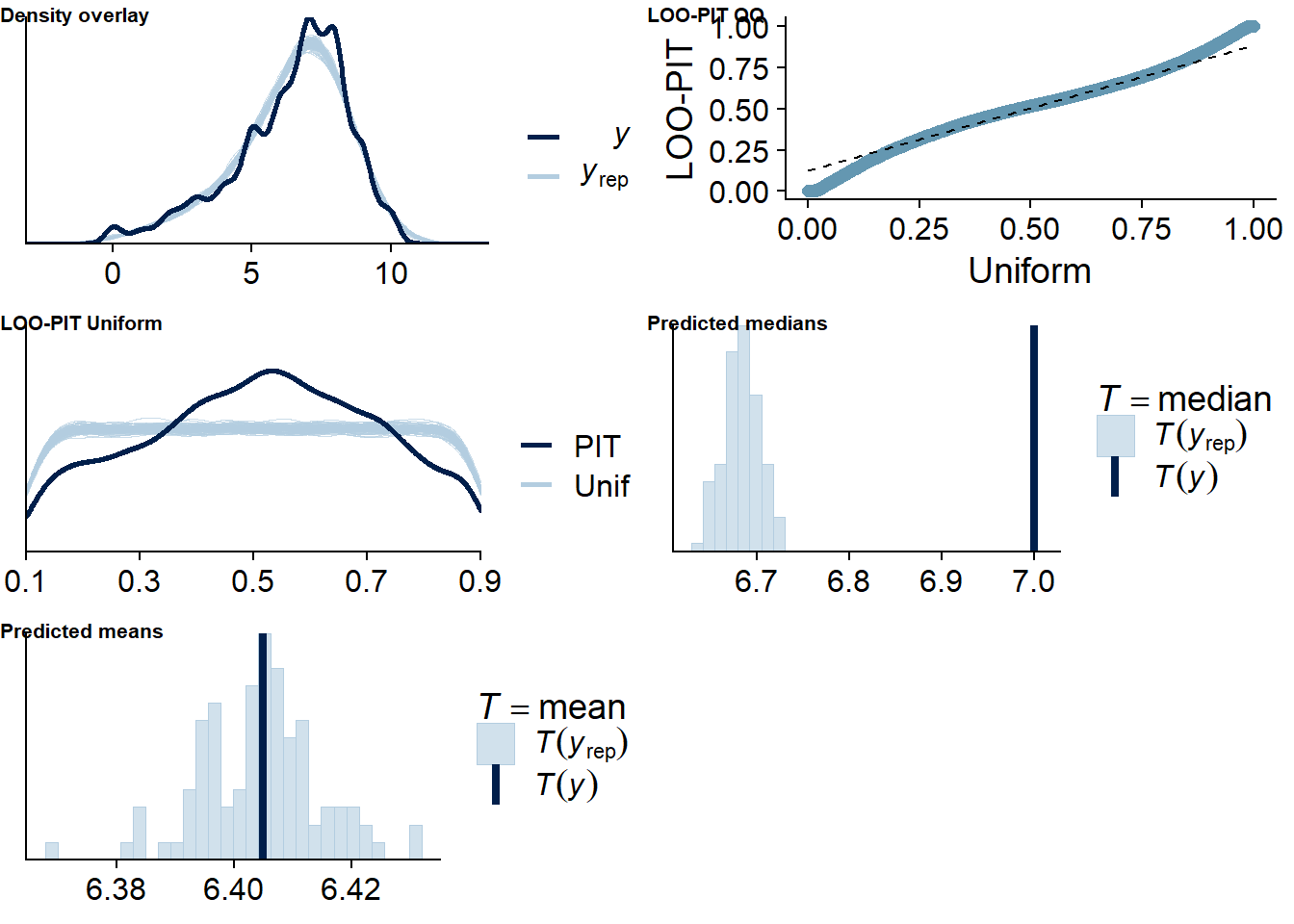
Figure 4.46: Posterior predictive checks for Films-Life Satisfaction model
The outliers are in about the same range as in previous models, and the model diagnostics look good.
films_life_loo <- loo(films_life)
films_life_loo
##
## Computed from 12000 by 10985 log-likelihood matrix
##
## Estimate SE
## elpd_loo -14553.5 146.7
## p_loo 2240.4 52.1
## looic 29107.0 293.4
## ------
## Monte Carlo SE of elpd_loo is NA.
##
## Pareto k diagnostic values:
## Count Pct. Min. n_eff
## (-Inf, 0.5] (good) 10339 94.1% 487
## (0.5, 0.7] (ok) 519 4.7% 114
## (0.7, 1] (bad) 114 1.0% 14
## (1, Inf) (very bad) 13 0.1% 5
## See help('pareto-k-diagnostic') for details.Below the summary.
summary(films_life)## Family: gaussian
## Links: mu = identity; sigma = identity
## Formula: life_satisfaction ~ 1 + films_used_between + films_used_within + films_time_between + films_time_within + (1 + films_time_within + films_used_within | id)
## Data: working_file (Number of observations: 10985)
## Samples: 4 chains, each with iter = 5000; warmup = 2000; thin = 1;
## total post-warmup samples = 12000
##
## Group-Level Effects:
## ~id (Number of levels: 2159)
## Estimate Est.Error l-95% CI u-95% CI Rhat Bulk_ESS Tail_ESS
## sd(Intercept) 1.91 0.03 1.85 1.97 1.00 924 1863
## sd(films_time_within) 0.08 0.01 0.05 0.10 1.00 2431 5028
## sd(films_used_within) 0.40 0.09 0.21 0.56 1.01 653 1783
## cor(Intercept,films_time_within) -0.03 0.11 -0.25 0.18 1.00 11830 8765
## cor(Intercept,films_used_within) 0.10 0.11 -0.10 0.32 1.00 9109 5304
## cor(films_time_within,films_used_within) 0.17 0.36 -0.43 0.88 1.01 521 1424
##
## Population-Level Effects:
## Estimate Est.Error l-95% CI u-95% CI Rhat Bulk_ESS Tail_ESS
## Intercept 6.53 0.09 6.36 6.72 1.00 795 1278
## films_used_between -0.18 0.14 -0.44 0.09 1.00 686 1316
## films_used_within 0.02 0.04 -0.06 0.10 1.00 16662 9772
## films_time_between 0.00 0.02 -0.04 0.05 1.00 871 1905
## films_time_within 0.00 0.01 -0.01 0.02 1.00 12798 9452
##
## Family Specific Parameters:
## Estimate Est.Error l-95% CI u-95% CI Rhat Bulk_ESS Tail_ESS
## sigma 0.80 0.01 0.79 0.82 1.00 7153 8760
##
## Samples were drawn using sampling(NUTS). For each parameter, Bulk_ESS
## and Tail_ESS are effective sample size measures, and Rhat is the potential
## scale reduction factor on split chains (at convergence, Rhat = 1).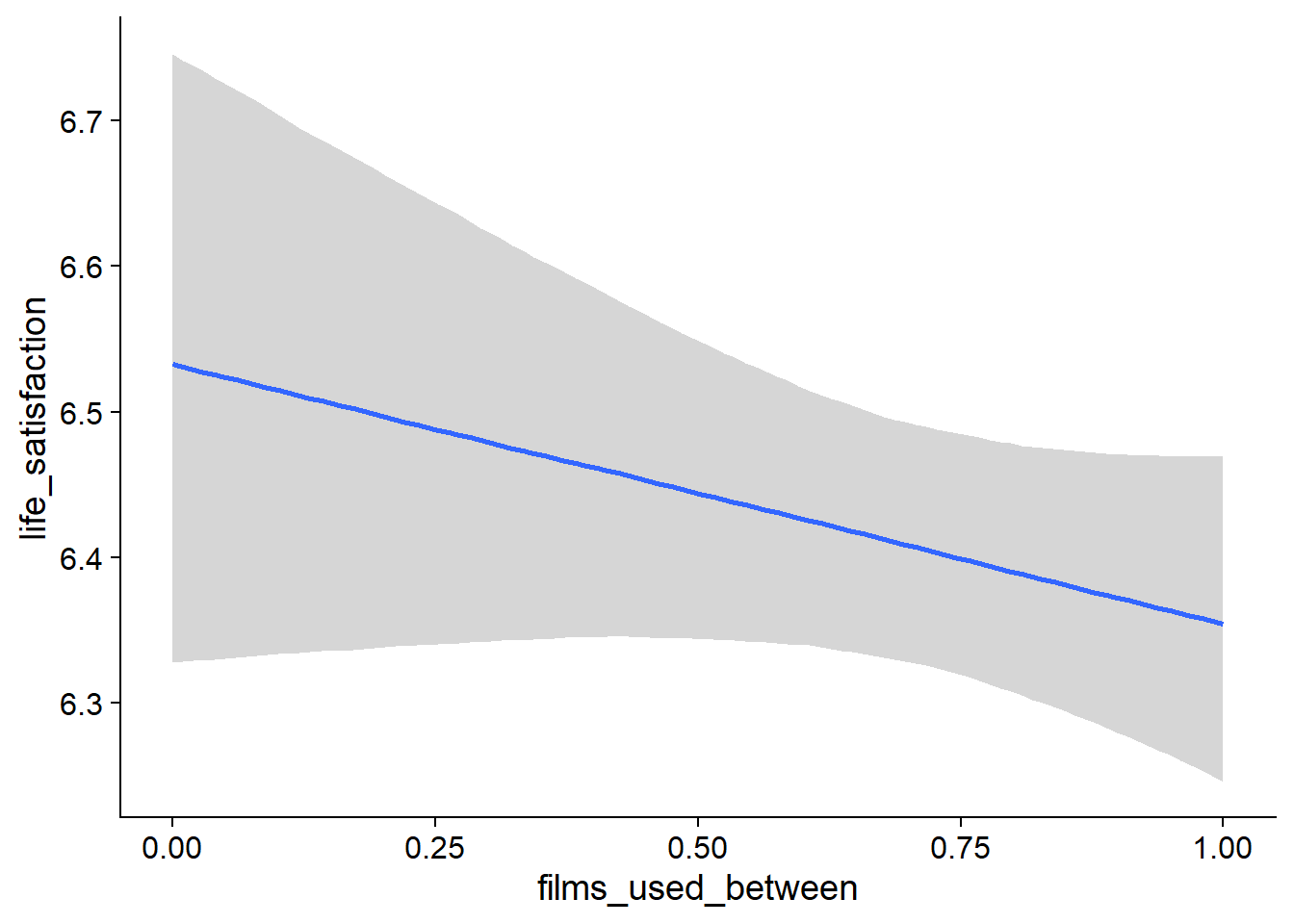
Figure 4.47: Conditional effects for Films-Life Satisfaction model
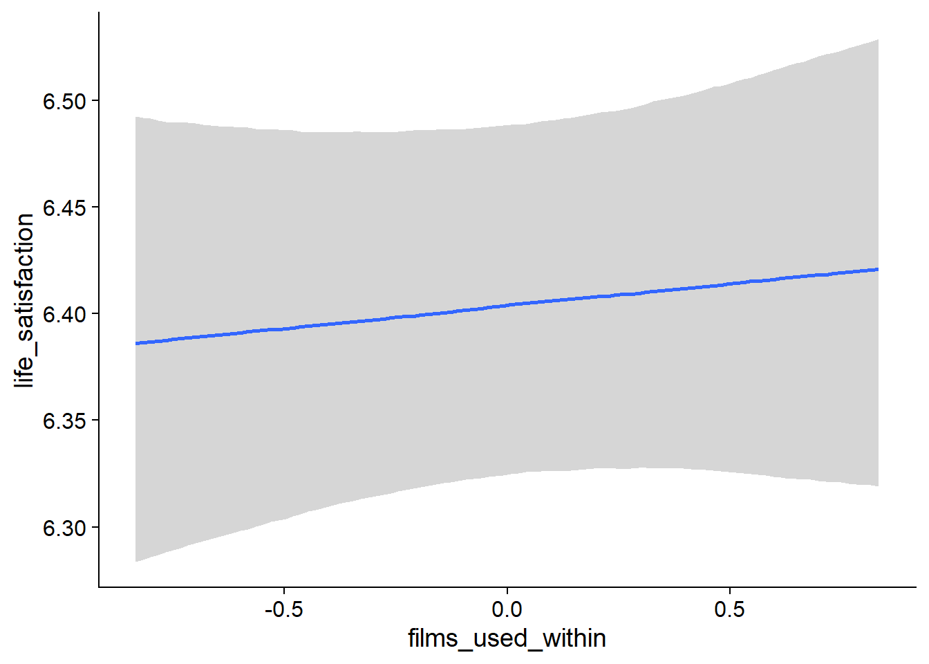
Figure 4.48: Conditional effects for Films-Life Satisfaction model
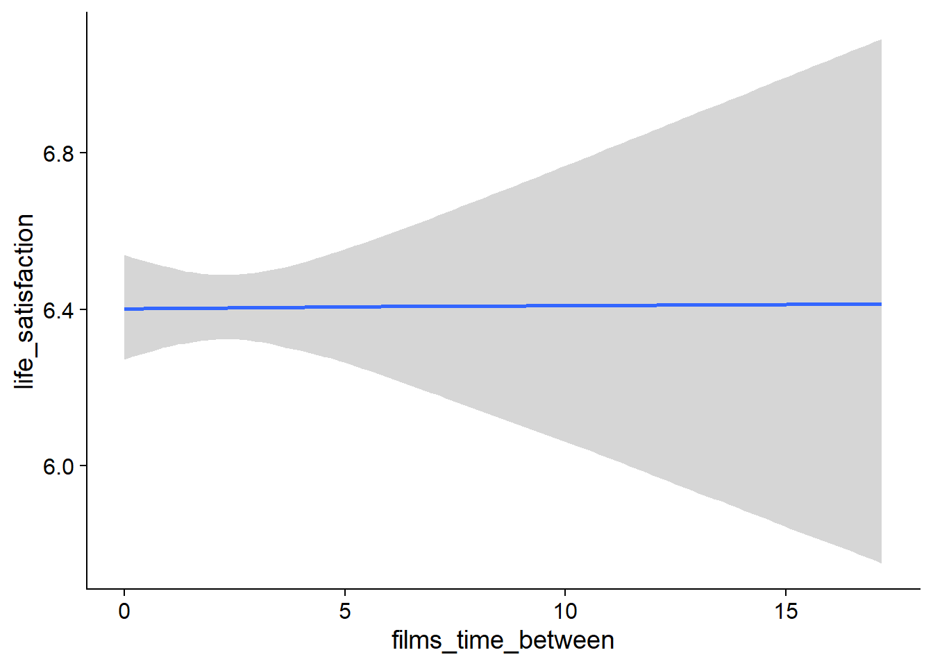
Figure 4.49: Conditional effects for Films-Life Satisfaction model
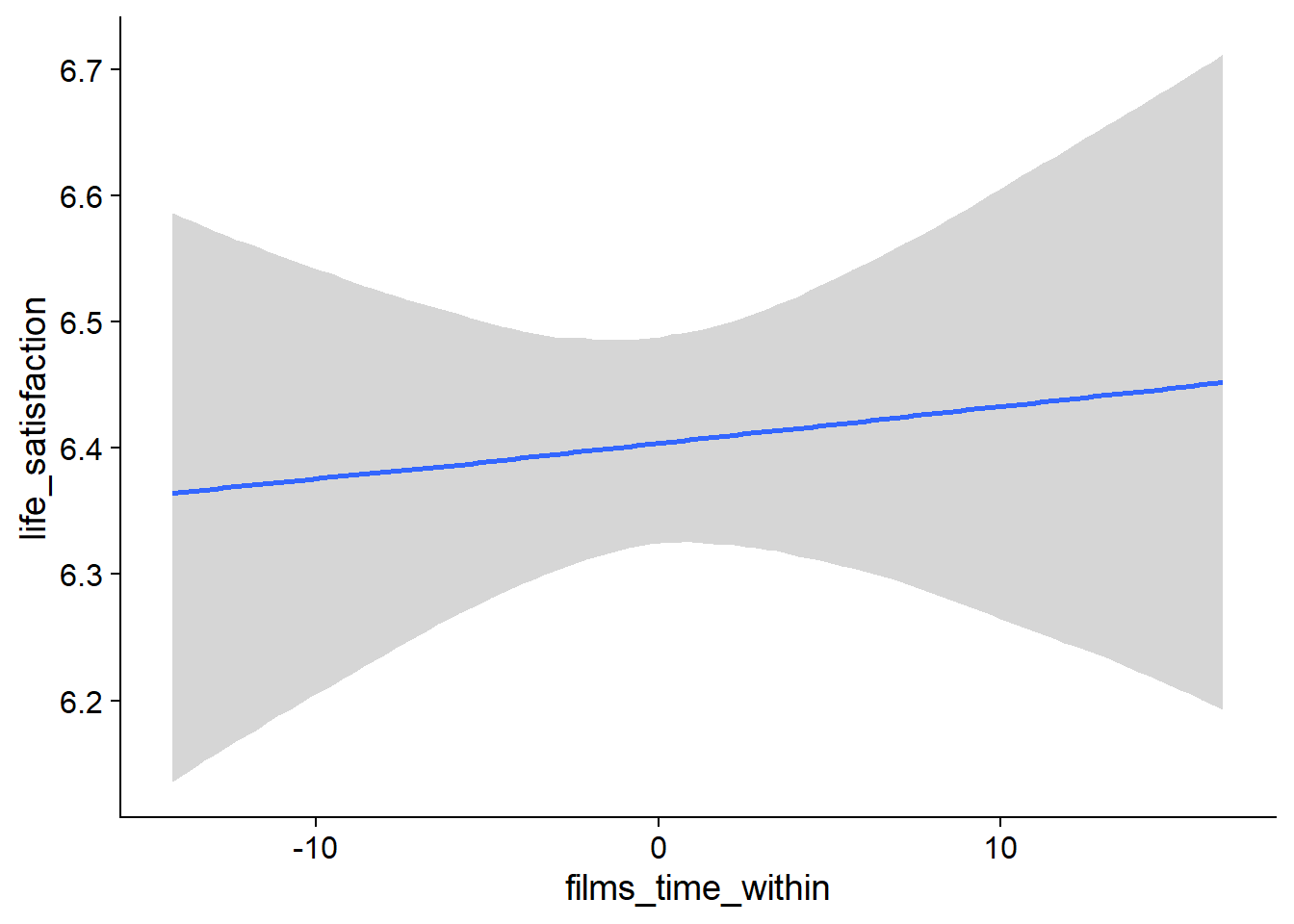
Figure 4.50: Conditional effects for Films-Life Satisfaction model
##            used  (Mb) gc trigger   (Mb)  max used   (Mb)
## Ncells  3692153 197.2    6044351  322.9   6044351  322.9
## Vcells 23771130 181.4  147932725 1128.7 221148237 1687.3
4.3.2.2 Life satisfaction on films
life_films <-
  brm(
    bf(
      # predicting continuous part
      lead_films_time ~
        1 +
        life_satisfaction_between +
        life_satisfaction_within +
        (1 +
           life_satisfaction_within
         | id),

      # predicting hurdle part
      hu ~
        1 +
        life_satisfaction_between +
        life_satisfaction_within +
        (1 +
           life_satisfaction_within
         | id)
    ),
    data = working_file,
    family = hurdle_gamma(),
    ,
    iter = 5000,
    warmup = 2000,
    chains = 4,
    cores = 4,
    seed = 42,
    control = list(adapt_delta = 0.95),
    file = here("models", "life_films")
  )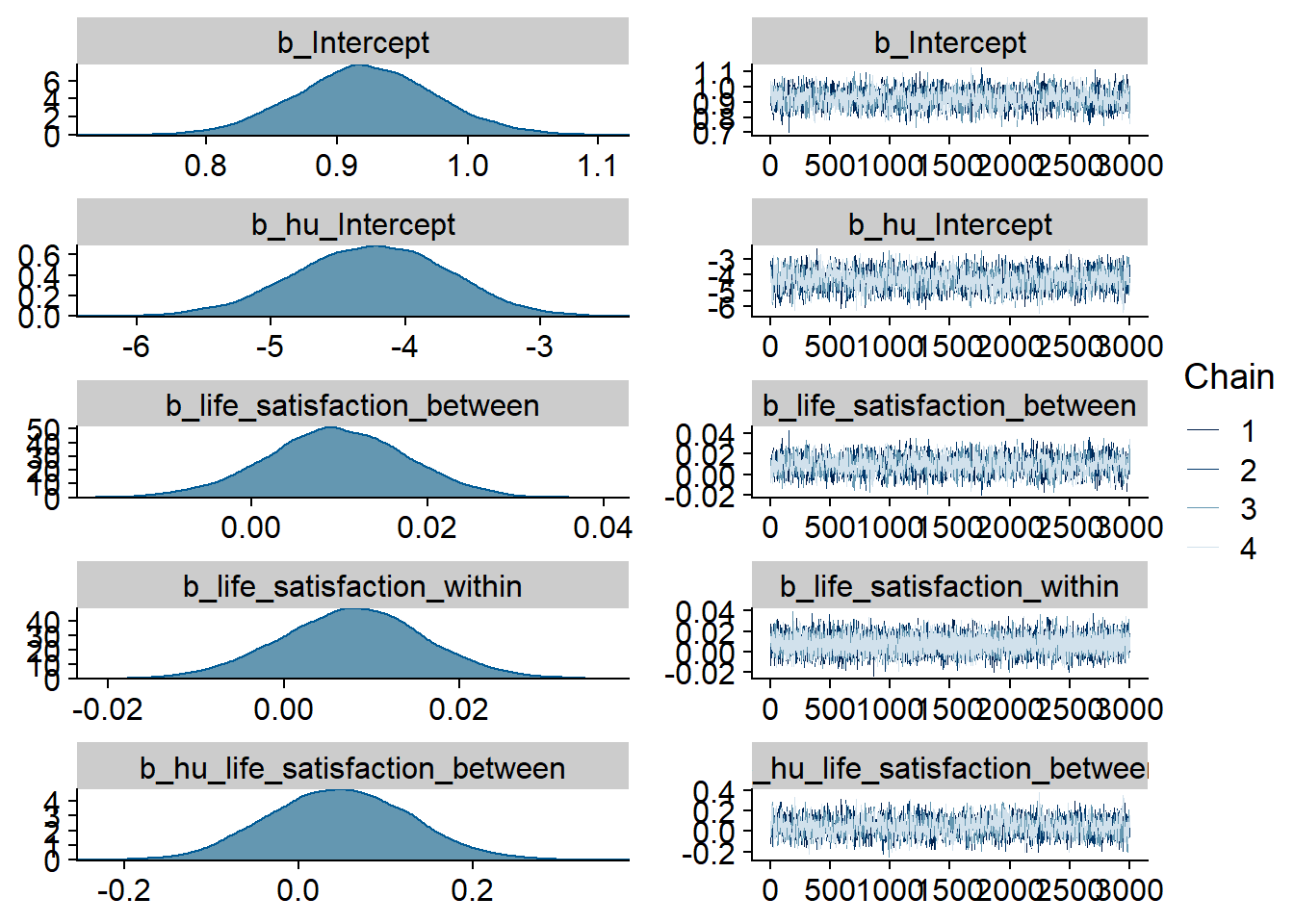
Figure 4.51: Traceplots and posterior distributions for Life Satisfaction-Films model
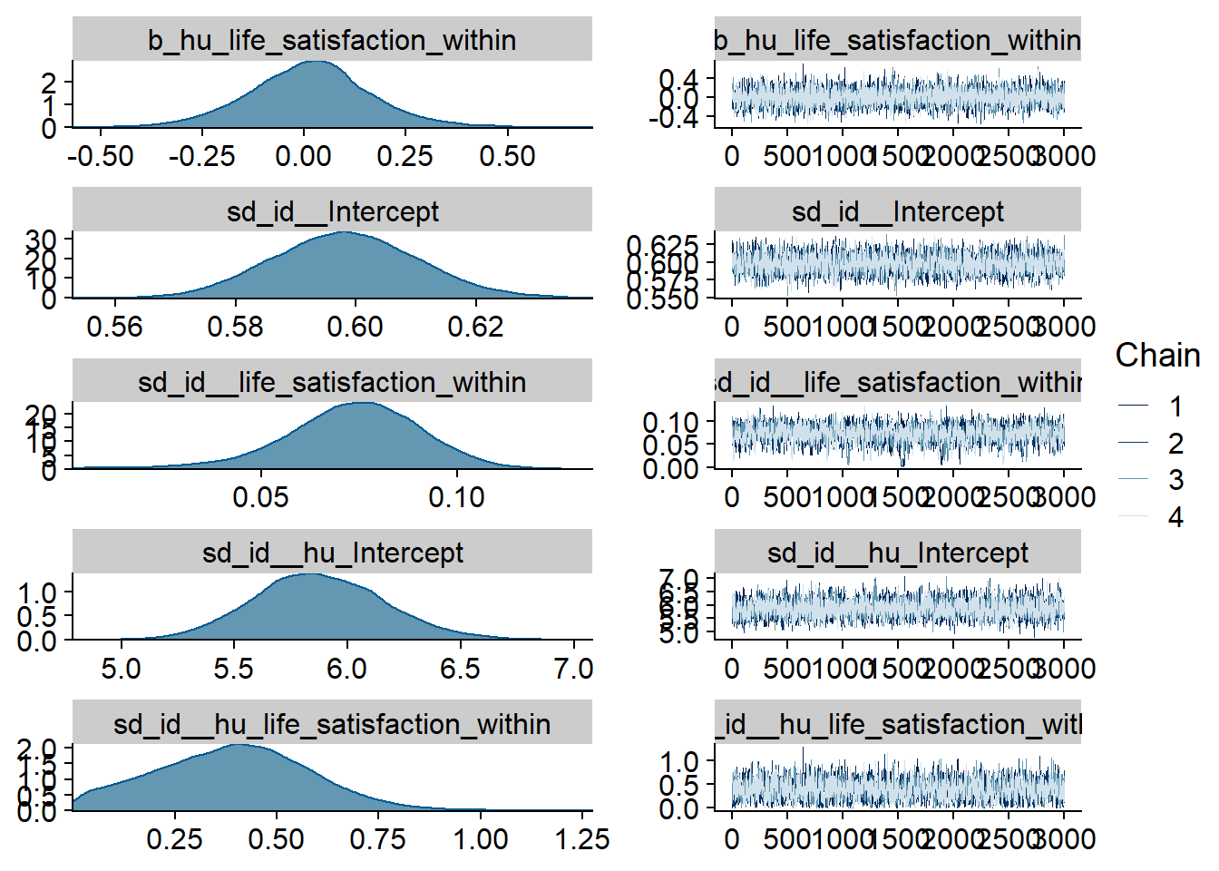
Figure 4.52: Traceplots and posterior distributions for Life Satisfaction-Films model
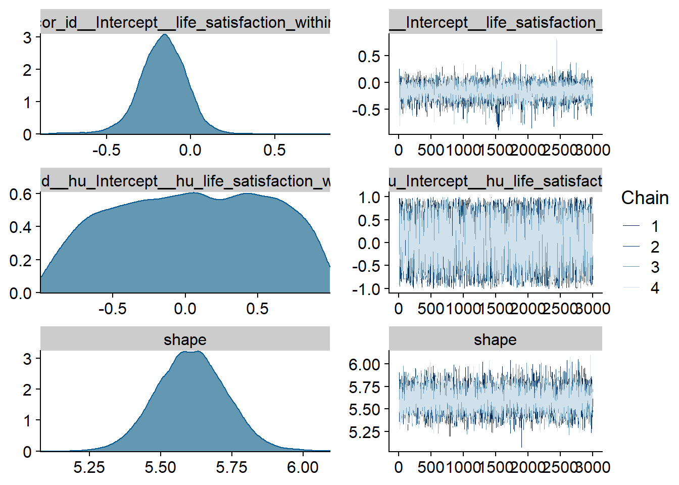
Figure 4.53: Traceplots and posterior distributions for Life Satisfaction-Films model
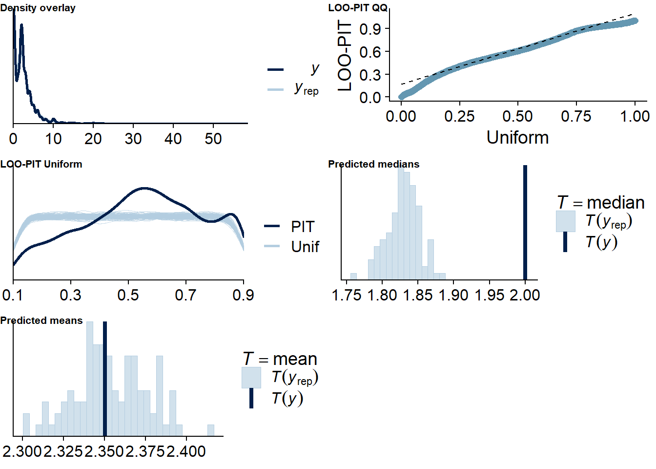
Figure 4.54: Posterior predictive checks for Life Satisfaction-Films model
The outliers are in about the same range as in previous models, and the model diagnostics look good.
life_films_loo <- loo(life_films)
life_films_loo
##
## Computed from 12000 by 8698 log-likelihood matrix
##
## Estimate SE
## elpd_loo -12636.2 129.4
## p_loo 2313.2 52.0
## looic 25272.4 258.7
## ------
## Monte Carlo SE of elpd_loo is NA.
##
## Pareto k diagnostic values:
## Count Pct. Min. n_eff
## (-Inf, 0.5] (good) 7543 86.7% 513
## (0.5, 0.7] (ok) 687 7.9% 136
## (0.7, 1] (bad) 400 4.6% 17
## (1, Inf) (very bad) 68 0.8% 1
## See help('pareto-k-diagnostic') for details.Below the summary.
summary(life_films)## Family: hurdle_gamma
## Links: mu = log; shape = identity; hu = logit
## Formula: lead_films_time ~ 1 + life_satisfaction_between + life_satisfaction_within + (1 + life_satisfaction_within | id)
## hu ~ 1 + life_satisfaction_between + life_satisfaction_within + (1 + life_satisfaction_within | id)
## Data: working_file (Number of observations: 8698)
## Samples: 4 chains, each with iter = 5000; warmup = 2000; thin = 1;
## total post-warmup samples = 12000
##
## Group-Level Effects:
## ~id (Number of levels: 2157)
## Estimate Est.Error l-95% CI u-95% CI Rhat Bulk_ESS Tail_ESS
## sd(Intercept) 0.60 0.01 0.58 0.62 1.00 3018 5935
## sd(life_satisfaction_within) 0.07 0.02 0.03 0.10 1.00 1290 1436
## sd(hu_Intercept) 5.87 0.29 5.33 6.46 1.00 3227 5686
## sd(hu_life_satisfaction_within) 0.39 0.19 0.04 0.76 1.00 1916 3118
## cor(Intercept,life_satisfaction_within) -0.17 0.14 -0.46 0.09 1.00 4802 2405
## cor(hu_Intercept,hu_life_satisfaction_within) 0.05 0.52 -0.87 0.91 1.00 5438 5421
##
## Population-Level Effects:
## Estimate Est.Error l-95% CI u-95% CI Rhat Bulk_ESS Tail_ESS
## Intercept 0.92 0.05 0.82 1.03 1.00 1838 3301
## hu_Intercept -4.26 0.57 -5.40 -3.18 1.00 1927 3638
## life_satisfaction_between 0.01 0.01 -0.01 0.03 1.00 1783 2987
## life_satisfaction_within 0.01 0.01 -0.01 0.02 1.00 12701 10479
## hu_life_satisfaction_between 0.05 0.08 -0.11 0.21 1.00 1947 3371
## hu_life_satisfaction_within 0.01 0.15 -0.29 0.32 1.00 5537 7355
##
## Family Specific Parameters:
## Estimate Est.Error l-95% CI u-95% CI Rhat Bulk_ESS Tail_ESS
## shape 5.61 0.12 5.37 5.85 1.00 4922 7087
##
## Samples were drawn using sampling(NUTS). For each parameter, Bulk_ESS
## and Tail_ESS are effective sample size measures, and Rhat is the potential
## scale reduction factor on split chains (at convergence, Rhat = 1).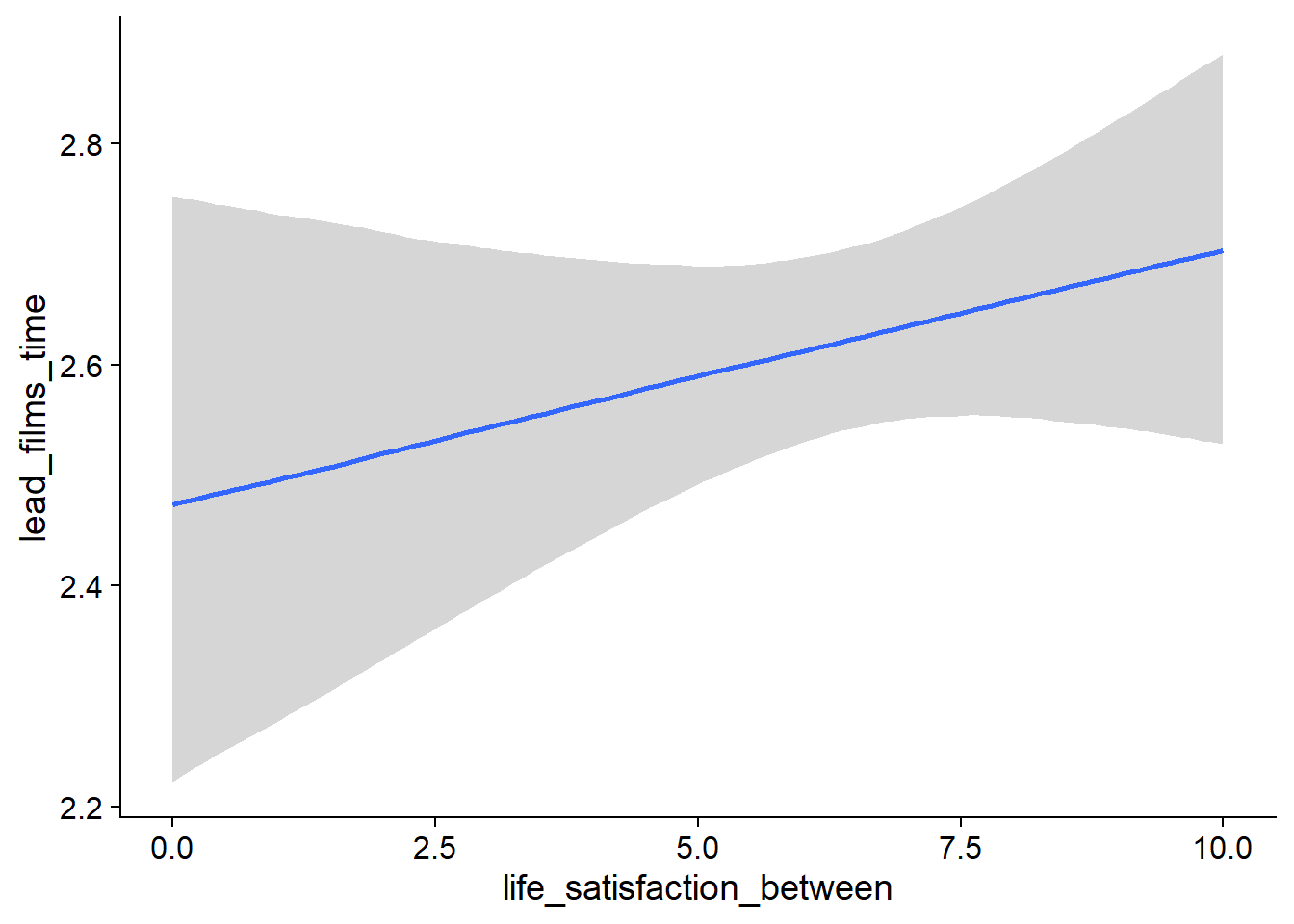
Figure 4.55: Conditional effects for Life Satisfaction-Films model
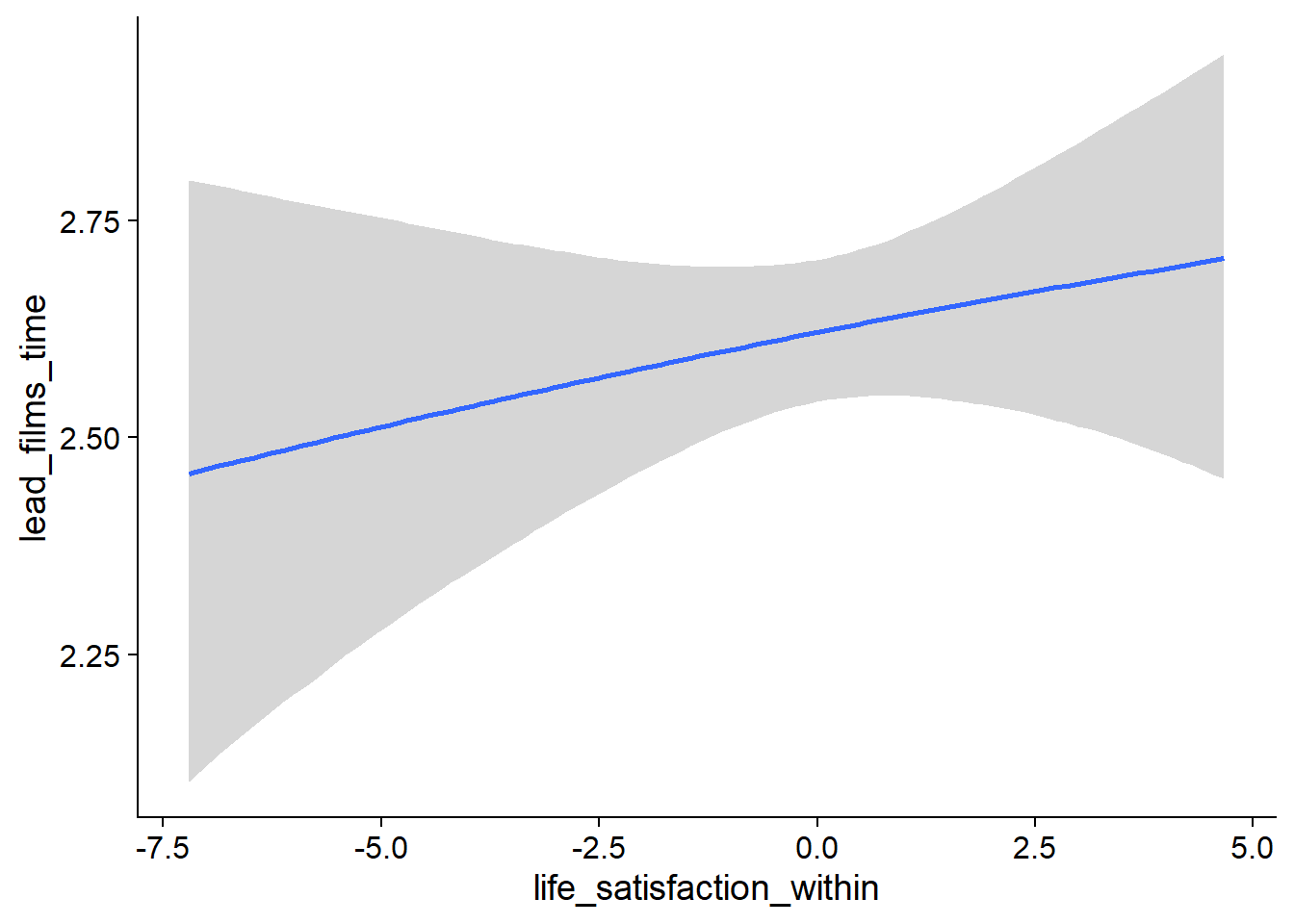
Figure 4.56: Conditional effects for Life Satisfaction-Films model
##            used  (Mb) gc trigger   (Mb)  max used   (Mb)
## Ncells  3692226 197.2    6044351  322.9   6044351  322.9
## Vcells 23772078 181.4  174110332 1328.4 221148237 1687.3
4.4 TV
4.4.1 Affect
4.4.1.1 TV on affect
tv_affect <-
  brm(
    data = working_file,
    family = gaussian,
    affect ~
      1 +
      tv_used_between +
      tv_used_within +
      tv_time_between +
      tv_time_within +
      (1 +
         tv_time_within +
         tv_used_within
       | id),
    iter = 5000,
    warmup = 2000,
    chains = 4,
    cores = 4,
    seed = 42,
    control = list(adapt_delta = 0.95),
    file = here("models", "tv_affect")
  )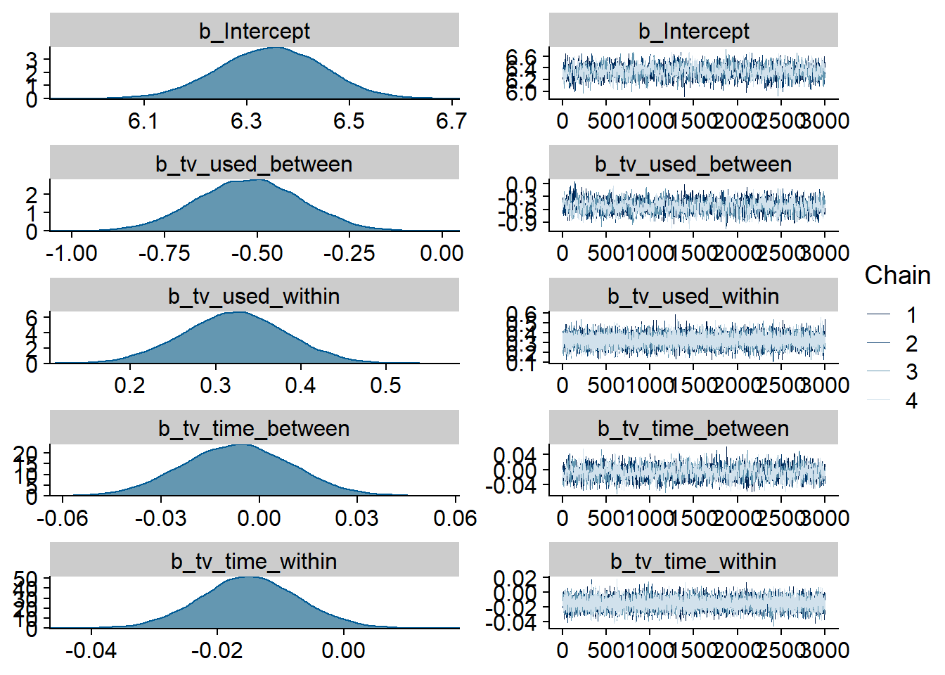
Figure 4.57: Traceplots and posterior distributions for TV-affect model
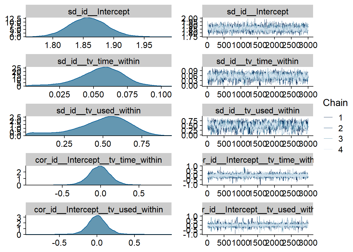
Figure 4.58: Traceplots and posterior distributions for TV-affect model
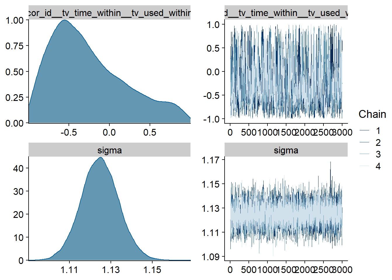
Figure 4.59: Traceplots and posterior distributions for TV-affect model
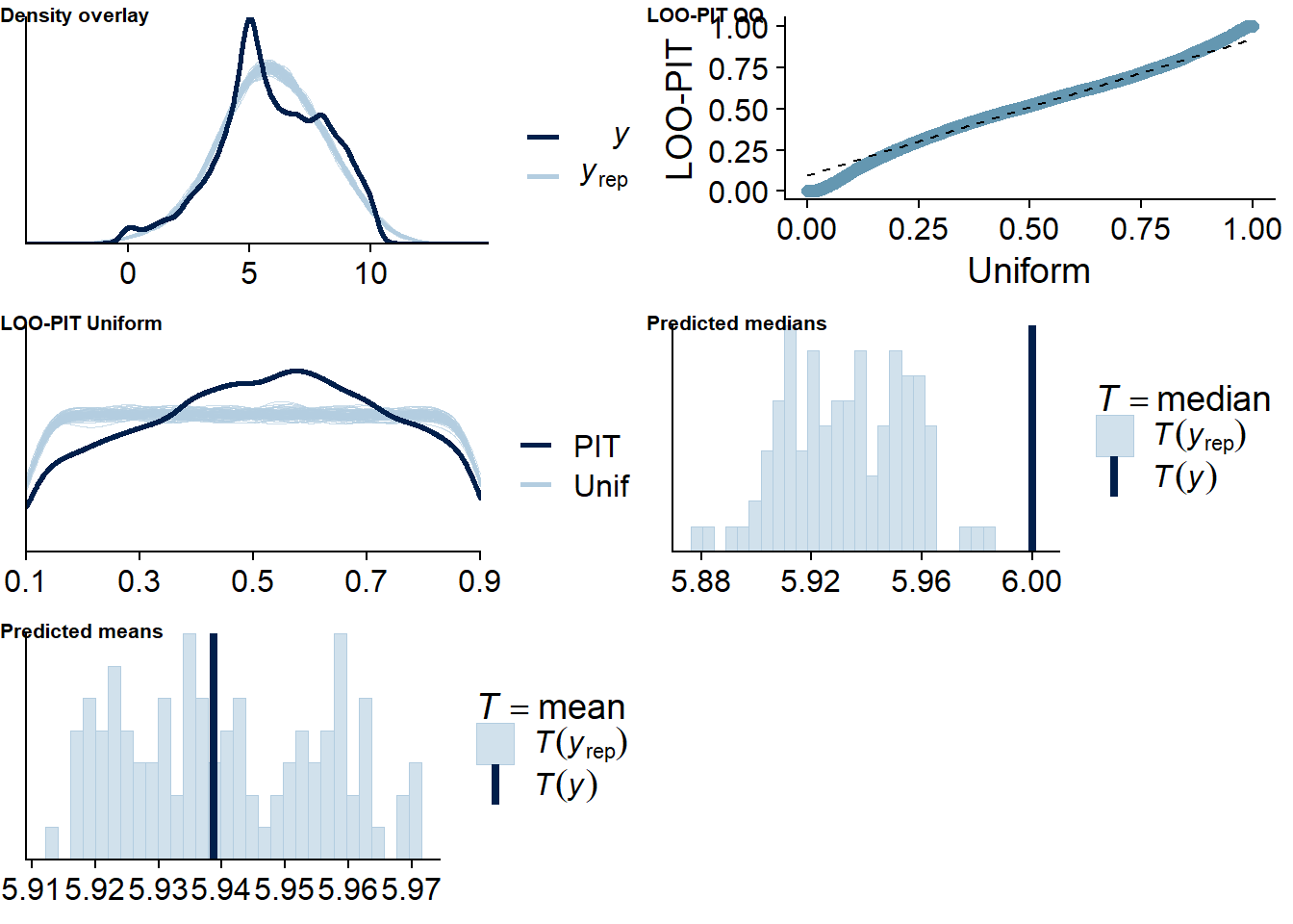
Figure 4.60: Posterior predictive checks for TV-affect model
The outliers are in about the same range as in previous models, and the model diagnostics look good.
tv_affect_loo <- loo(tv_affect)
tv_affect_loo
##
## Computed from 12000 by 10985 log-likelihood matrix
##
## Estimate SE
## elpd_loo -18088.1 105.3
## p_loo 2022.1 35.4
## looic 36176.2 210.7
## ------
## Monte Carlo SE of elpd_loo is NA.
##
## Pareto k diagnostic values:
## Count Pct. Min. n_eff
## (-Inf, 0.5] (good) 10549 96.0% 531
## (0.5, 0.7] (ok) 387 3.5% 108
## (0.7, 1] (bad) 47 0.4% 27
## (1, Inf) (very bad) 2 0.0% 4
## See help('pareto-k-diagnostic') for details.Below the summary.
summary(tv_affect)## Family: gaussian
## Links: mu = identity; sigma = identity
## Formula: affect ~ 1 + tv_used_between + tv_used_within + tv_time_between + tv_time_within + (1 + tv_time_within + tv_used_within | id)
## Data: working_file (Number of observations: 10985)
## Samples: 4 chains, each with iter = 5000; warmup = 2000; thin = 1;
## total post-warmup samples = 12000
##
## Group-Level Effects:
## ~id (Number of levels: 2159)
## Estimate Est.Error l-95% CI u-95% CI Rhat Bulk_ESS Tail_ESS
## sd(Intercept) 1.86 0.03 1.80 1.92 1.00 2338 4271
## sd(tv_time_within) 0.06 0.02 0.02 0.09 1.00 1606 1396
## sd(tv_used_within) 0.49 0.18 0.06 0.77 1.01 655 904
## cor(Intercept,tv_time_within) -0.02 0.16 -0.32 0.28 1.00 9556 4271
## cor(Intercept,tv_used_within) 0.01 0.16 -0.29 0.33 1.00 6971 2509
## cor(tv_time_within,tv_used_within) -0.26 0.46 -0.92 0.80 1.00 669 1682
##
## Population-Level Effects:
## Estimate Est.Error l-95% CI u-95% CI Rhat Bulk_ESS Tail_ESS
## Intercept 6.35 0.10 6.15 6.54 1.00 1670 3232
## tv_used_between -0.52 0.14 -0.79 -0.25 1.00 1536 3120
## tv_used_within 0.32 0.06 0.20 0.44 1.00 19453 10357
## tv_time_between -0.01 0.02 -0.04 0.03 1.00 1638 3115
## tv_time_within -0.01 0.01 -0.03 0.00 1.00 17512 10735
##
## Family Specific Parameters:
## Estimate Est.Error l-95% CI u-95% CI Rhat Bulk_ESS Tail_ESS
## sigma 1.12 0.01 1.11 1.14 1.00 7251 9895
##
## Samples were drawn using sampling(NUTS). For each parameter, Bulk_ESS
## and Tail_ESS are effective sample size measures, and Rhat is the potential
## scale reduction factor on split chains (at convergence, Rhat = 1).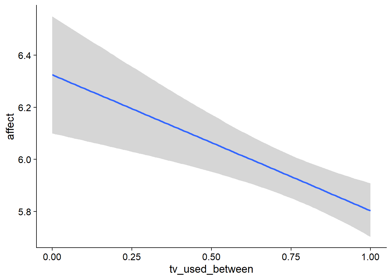
Figure 4.61: Conditional effects for TV-affect model
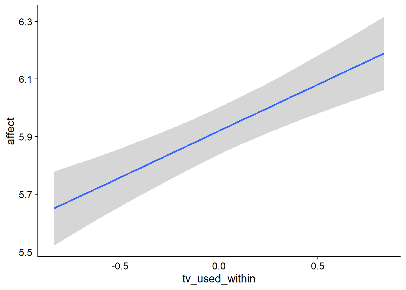
Figure 4.62: Conditional effects for TV-affect model
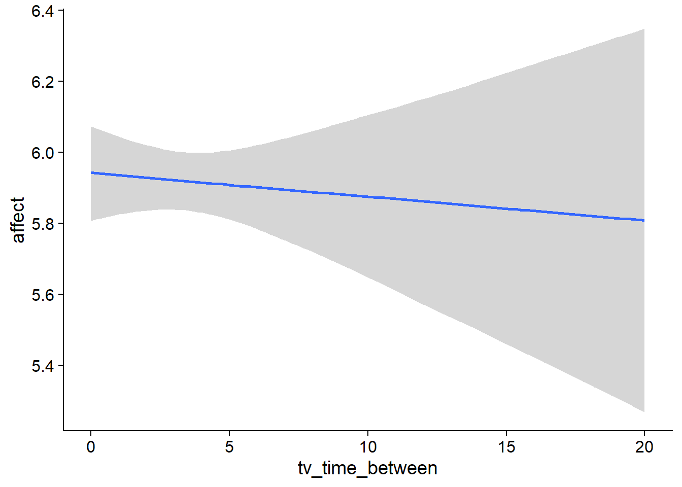
Figure 4.63: Conditional effects for TV-affect model
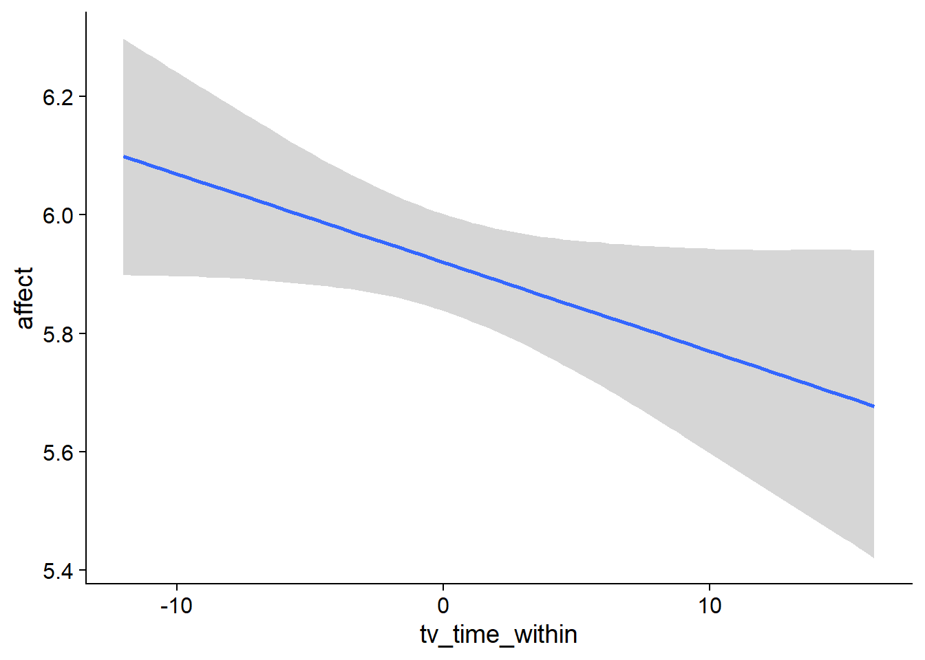
Figure 4.64: Conditional effects for TV-affect model
##            used  (Mb) gc trigger   (Mb)  max used   (Mb)
## Ncells  3692344 197.2    6044351  322.9   6044351  322.9
## Vcells 23773042 181.4  139288266 1062.7 221148237 1687.3
4.4.1.2 Affect on TV
affect_tv <-
  brm(
    bf(
      # predicting continuous part
      lead_tv_time ~
        1 +
        affect_between +
        affect_within +
        (1 +
           affect_within
         | id),

      # predicting hurdle part
      hu ~
        1 +
        affect_between +
        affect_within +
        (1 +
           affect_within
         | id)
    ),
    data = working_file,
    family = hurdle_gamma(),
    ,
    iter = 5000,
    warmup = 2000,
    chains = 4,
    cores = 4,
    seed = 42,
    control = list(adapt_delta = 0.95),
    file = here("models", "affect_tv")
  )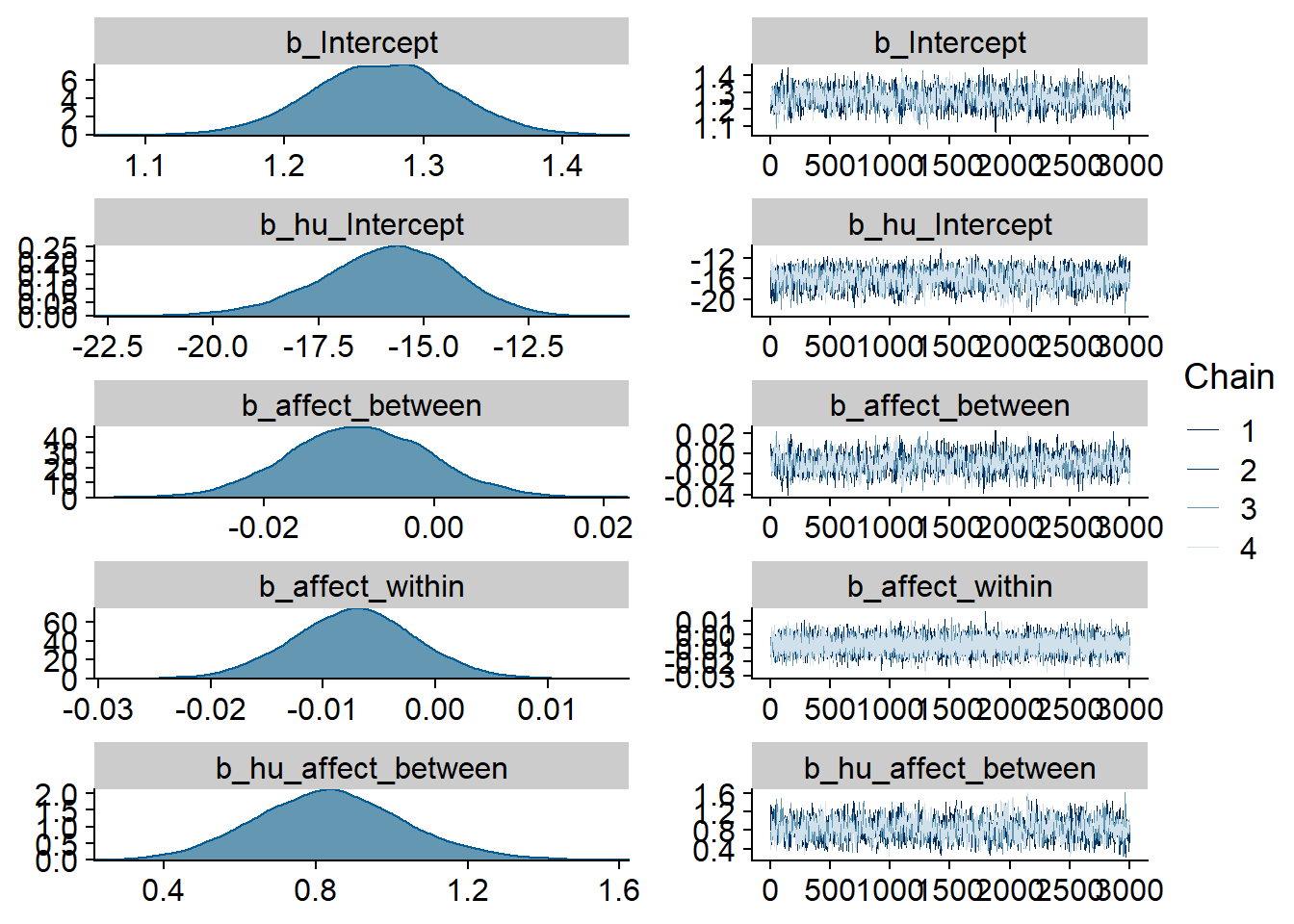
Figure 4.65: Traceplots and posterior distributions for Affect-TV model
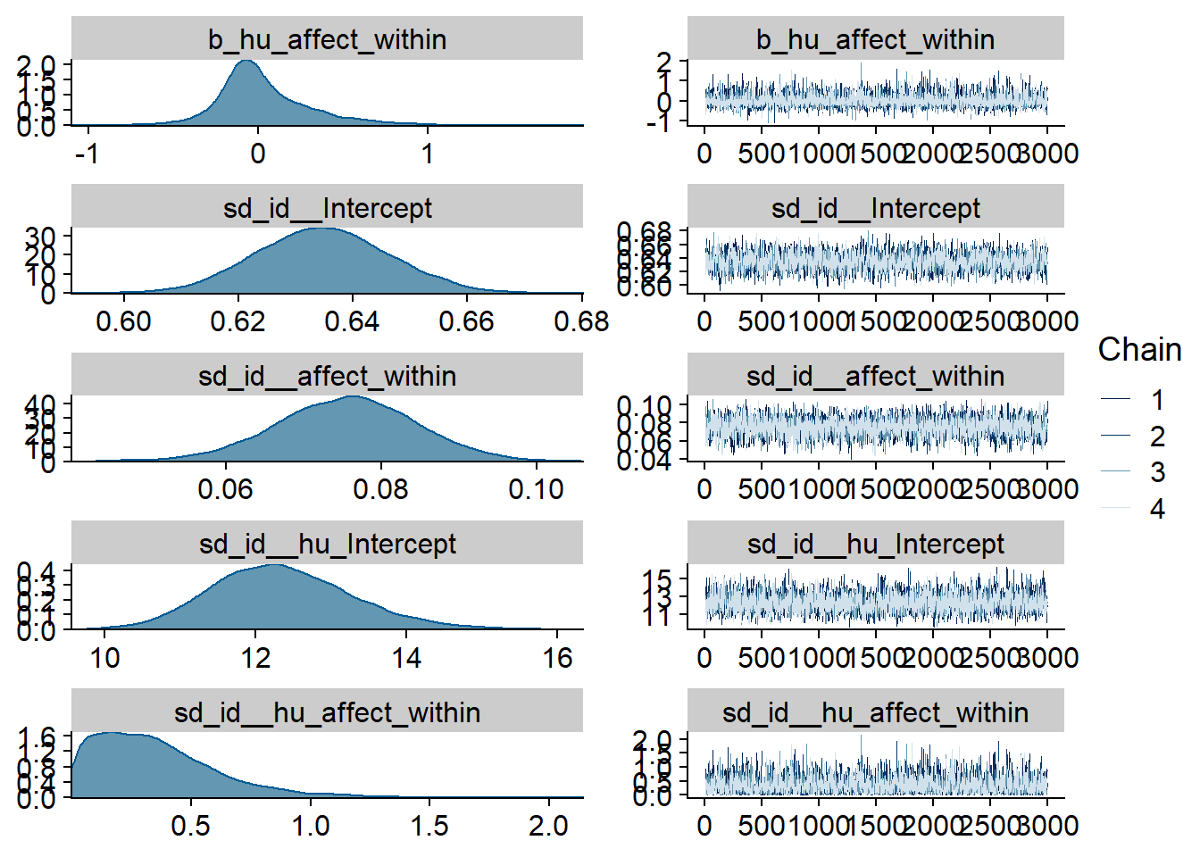
Figure 4.66: Traceplots and posterior distributions for Affect-TV model
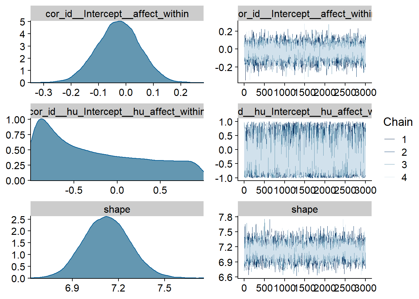
Figure 4.67: Traceplots and posterior distributions for Affect-TV model
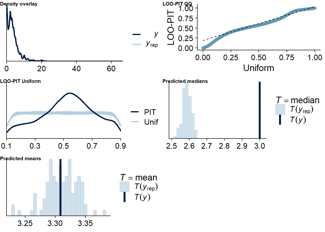
Figure 4.68: Posterior predictive checks for Affect-TV model
The outliers are in about the same range as in previous models, and the model diagnostics look good.
affect_tv_loo <- loo(affect_tv)
affect_tv_loo
##
## Computed from 12000 by 8698 log-likelihood matrix
##
## Estimate SE
## elpd_loo -13342.2 138.3
## p_loo 2106.3 55.7
## looic 26684.4 276.6
## ------
## Monte Carlo SE of elpd_loo is NA.
##
## Pareto k diagnostic values:
## Count Pct. Min. n_eff
## (-Inf, 0.5] (good) 7671 88.2% 517
## (0.5, 0.7] (ok) 649 7.5% 167
## (0.7, 1] (bad) 287 3.3% 17
## (1, Inf) (very bad) 91 1.0% 1
## See help('pareto-k-diagnostic') for details.Below the summary.
summary(affect_tv)## Family: hurdle_gamma
## Links: mu = log; shape = identity; hu = logit
## Formula: lead_tv_time ~ 1 + affect_between + affect_within + (1 + affect_within | id)
## hu ~ 1 + affect_between + affect_within + (1 + affect_within | id)
## Data: working_file (Number of observations: 8698)
## Samples: 4 chains, each with iter = 5000; warmup = 2000; thin = 1;
## total post-warmup samples = 12000
##
## Group-Level Effects:
## ~id (Number of levels: 2157)
## Estimate Est.Error l-95% CI u-95% CI Rhat Bulk_ESS Tail_ESS
## sd(Intercept) 0.63 0.01 0.61 0.66 1.00 2205 4586
## sd(affect_within) 0.08 0.01 0.06 0.09 1.00 2565 4401
## sd(hu_Intercept) 12.36 0.94 10.69 14.37 1.00 2990 5055
## sd(hu_affect_within) 0.35 0.26 0.02 1.02 1.00 2586 4882
## cor(Intercept,affect_within) -0.03 0.08 -0.18 0.12 1.00 10673 8894
## cor(hu_Intercept,hu_affect_within) -0.25 0.59 -0.98 0.91 1.00 6226 5652
##
## Population-Level Effects:
## Estimate Est.Error l-95% CI u-95% CI Rhat Bulk_ESS Tail_ESS
## Intercept 1.27 0.05 1.17 1.37 1.00 1429 2809
## hu_Intercept -15.87 1.61 -19.30 -12.91 1.00 1992 4123
## affect_between -0.01 0.01 -0.02 0.01 1.00 1363 2525
## affect_within -0.01 0.01 -0.02 0.00 1.00 14420 9042
## hu_affect_between 0.84 0.20 0.47 1.24 1.00 1709 3706
## hu_affect_within 0.03 0.28 -0.42 0.71 1.00 5071 5499
##
## Family Specific Parameters:
## Estimate Est.Error l-95% CI u-95% CI Rhat Bulk_ESS Tail_ESS
## shape 7.12 0.15 6.84 7.42 1.00 6449 8029
##
## Samples were drawn using sampling(NUTS). For each parameter, Bulk_ESS
## and Tail_ESS are effective sample size measures, and Rhat is the potential
## scale reduction factor on split chains (at convergence, Rhat = 1).
Figure 4.69: Conditional effects for Affect-TV model
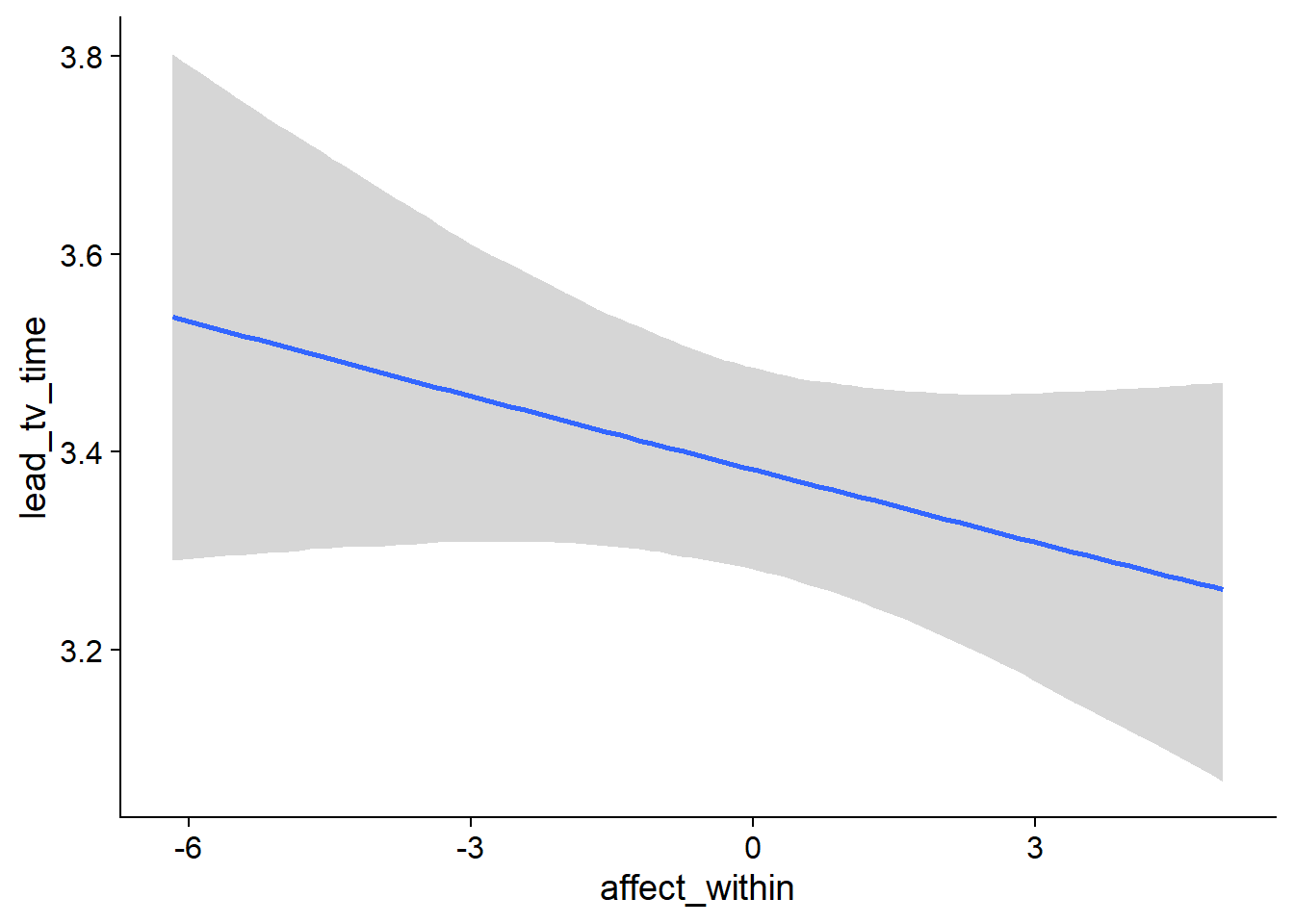
Figure 4.70: Conditional effects for Affect-TV model
##            used  (Mb) gc trigger   (Mb)  max used   (Mb)
## Ncells  3692441 197.2    6044351  322.9   6044351  322.9
## Vcells 23773948 181.4  197038620 1503.3 221148237 1687.3
4.4.2 Life satisfaction
4.4.2.1 TV on life satisfaction
tv_life <-
  brm(
    data = working_file,
    family = gaussian,
    life_satisfaction ~
      1 +
      tv_used_between +
      tv_used_within +
      tv_time_between +
      tv_time_within +
      (1 +
         tv_time_within +
         tv_used_within
       | id),
    iter = 5000,
    warmup = 2000,
    chains = 4,
    cores = 4,
    seed = 42,
    control = list(adapt_delta = 0.95),
    file = here("models", "tv_life")
  )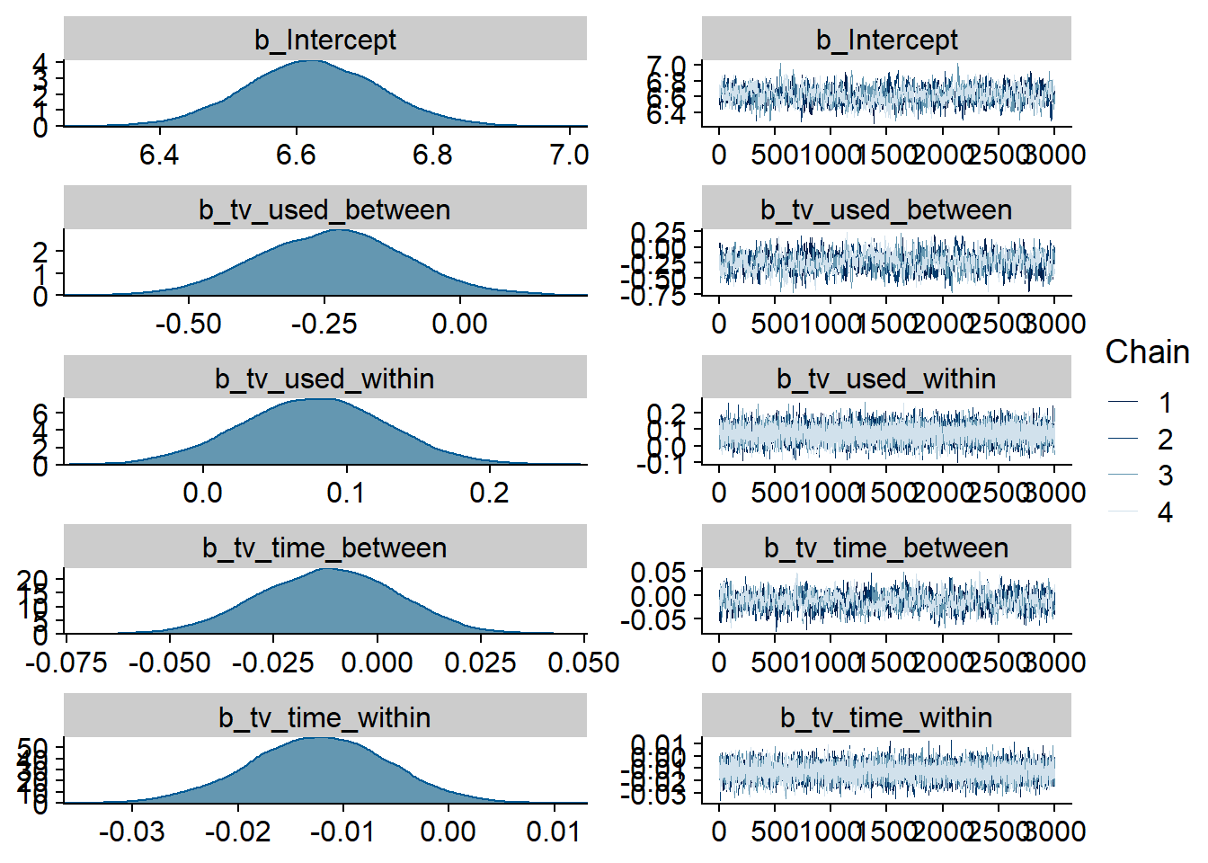
Figure 4.71: Traceplots and posterior distributions for TV-Life Satisfaction model
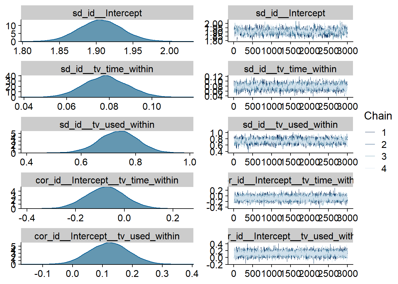
Figure 4.72: Traceplots and posterior distributions for TV-Life Satisfaction model
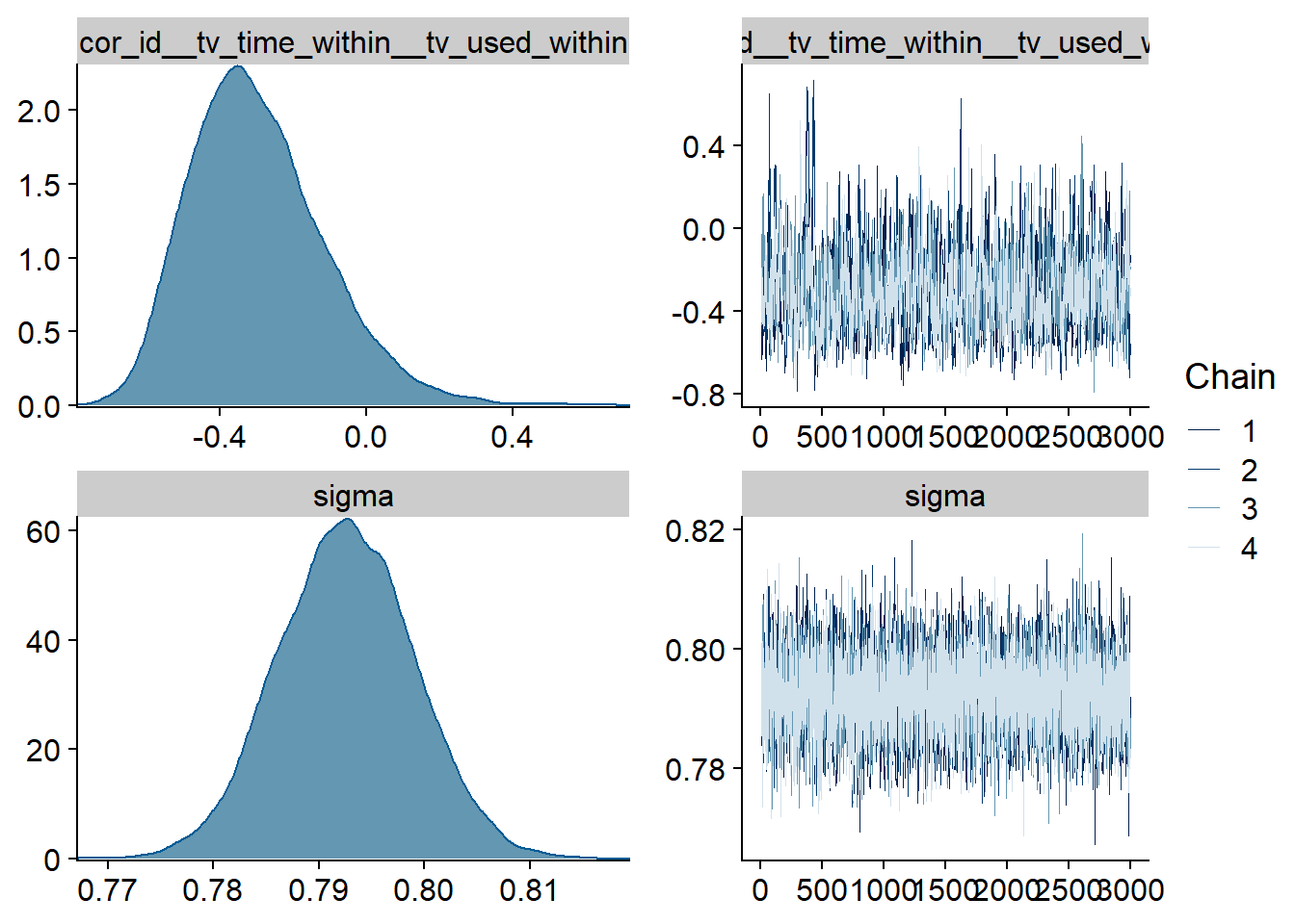
Figure 4.73: Traceplots and posterior distributions for TV-Life Satisfaction model
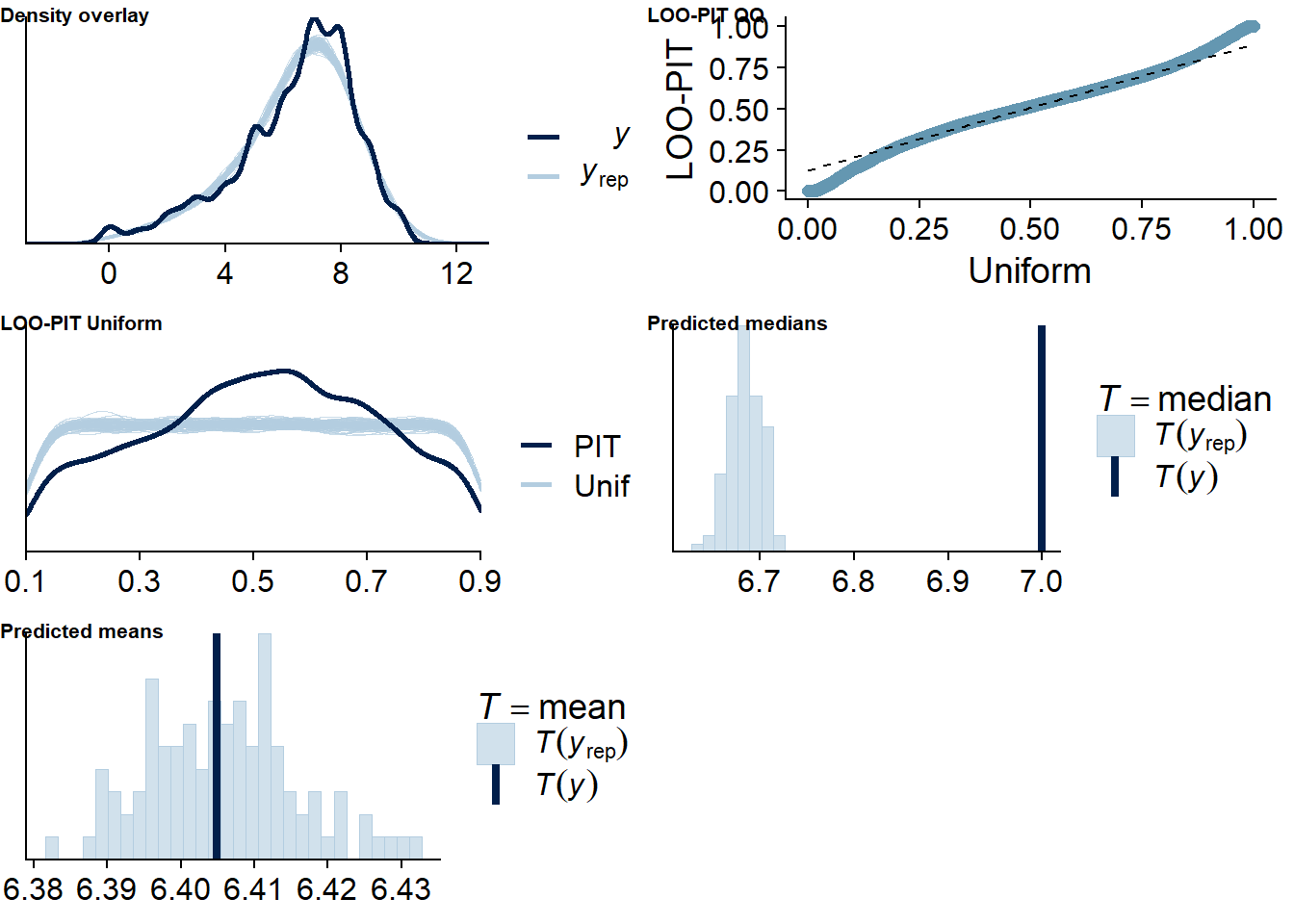
Figure 4.74: Posterior predictive checks for TV-Life Satisfaction model
The outliers are in about the same range as in previous models, and the model diagnostics look good.
tv_life_loo <- loo(tv_life)
tv_life_loo
##
## Computed from 12000 by 10985 log-likelihood matrix
##
## Estimate SE
## elpd_loo -14491.4 141.1
## p_loo 2350.7 53.3
## looic 28982.7 282.2
## ------
## Monte Carlo SE of elpd_loo is NA.
##
## Pareto k diagnostic values:
## Count Pct. Min. n_eff
## (-Inf, 0.5] (good) 10001 91.0% 580
## (0.5, 0.7] (ok) 775 7.1% 91
## (0.7, 1] (bad) 190 1.7% 12
## (1, Inf) (very bad) 19 0.2% 3
## See help('pareto-k-diagnostic') for details.Below the summary.
summary(tv_life)## Family: gaussian
## Links: mu = identity; sigma = identity
## Formula: life_satisfaction ~ 1 + tv_used_between + tv_used_within + tv_time_between + tv_time_within + (1 + tv_time_within + tv_used_within | id)
## Data: working_file (Number of observations: 10985)
## Samples: 4 chains, each with iter = 5000; warmup = 2000; thin = 1;
## total post-warmup samples = 12000
##
## Group-Level Effects:
## ~id (Number of levels: 2159)
## Estimate Est.Error l-95% CI u-95% CI Rhat Bulk_ESS Tail_ESS
## sd(Intercept) 1.91 0.03 1.85 1.97 1.00 1259 2194
## sd(tv_time_within) 0.08 0.01 0.06 0.10 1.00 2516 4556
## sd(tv_used_within) 0.74 0.07 0.59 0.87 1.00 1685 3079
## cor(Intercept,tv_time_within) -0.08 0.08 -0.23 0.08 1.00 11636 10011
## cor(Intercept,tv_used_within) 0.12 0.07 -0.01 0.25 1.00 9586 9190
## cor(tv_time_within,tv_used_within) -0.30 0.19 -0.59 0.12 1.00 979 1412
##
## Population-Level Effects:
## Estimate Est.Error l-95% CI u-95% CI Rhat Bulk_ESS Tail_ESS
## Intercept 6.62 0.10 6.43 6.82 1.00 790 1742
## tv_used_between -0.24 0.14 -0.50 0.03 1.00 734 1664
## tv_used_within 0.08 0.05 -0.02 0.18 1.00 13043 10030
## tv_time_between -0.01 0.02 -0.04 0.02 1.00 833 1834
## tv_time_within -0.01 0.01 -0.03 0.00 1.00 11460 10393
##
## Family Specific Parameters:
## Estimate Est.Error l-95% CI u-95% CI Rhat Bulk_ESS Tail_ESS
## sigma 0.79 0.01 0.78 0.81 1.00 9884 9895
##
## Samples were drawn using sampling(NUTS). For each parameter, Bulk_ESS
## and Tail_ESS are effective sample size measures, and Rhat is the potential
## scale reduction factor on split chains (at convergence, Rhat = 1).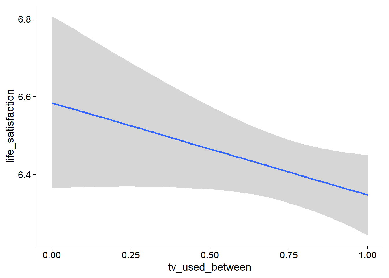
Figure 4.75: Conditional effects for TV-Life Satisfaction model
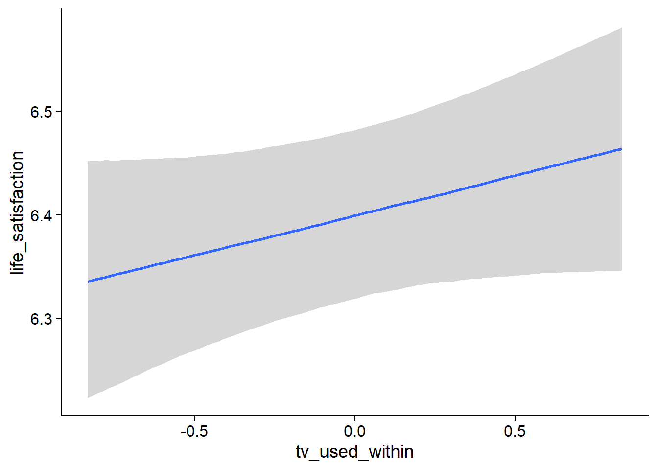
Figure 4.76: Conditional effects for TV-Life Satisfaction model
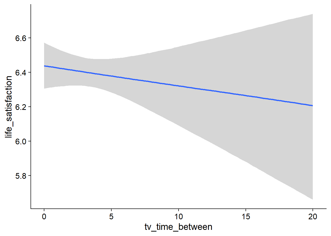
Figure 4.77: Conditional effects for TV-Life Satisfaction model
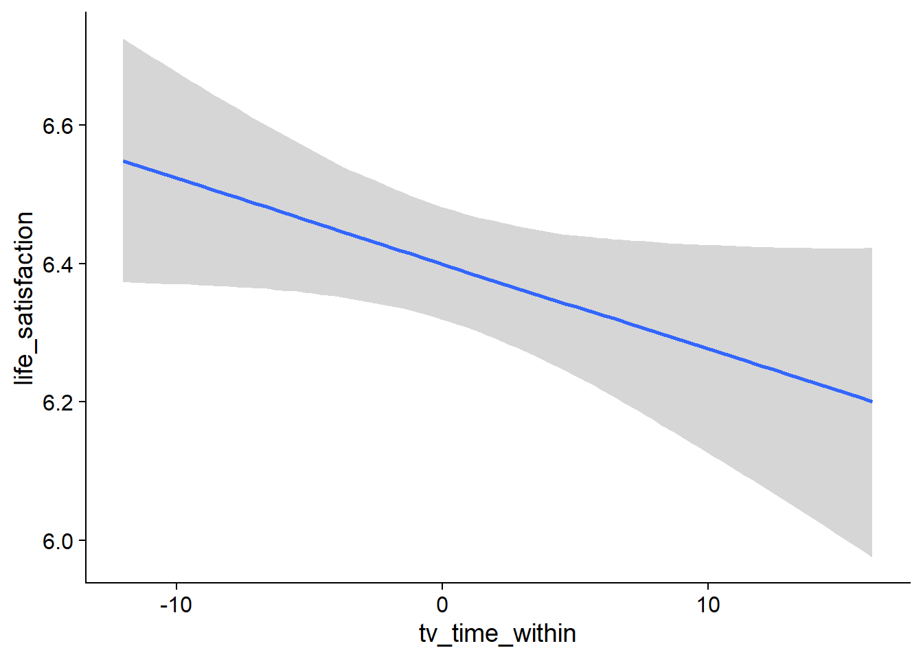
Figure 4.78: Conditional effects for TV-Life Satisfaction model
##            used  (Mb) gc trigger   (Mb)  max used   (Mb)
## Ncells  3692574 197.3    6044351  322.9   6044351  322.9
## Vcells 23774966 181.4  157630896 1202.7 221148237 1687.3
4.4.2.2 Life satisfaction on TV
life_tv <-
  brm(
    bf(
      # predicting continuous part
      lead_tv_time ~
        1 +
        life_satisfaction_between +
        life_satisfaction_within +
        (1 +
           life_satisfaction_within
         | id),

      # predicting hurdle part
      hu ~
        1 +
        life_satisfaction_between +
        life_satisfaction_within +
        (1 +
           life_satisfaction_within
         | id)
    ),
    data = working_file,
    family = hurdle_gamma(),
    ,
    iter = 5000,
    warmup = 2000,
    chains = 4,
    cores = 4,
    seed = 42,
    control = list(adapt_delta = 0.95),
    file = here("models", "life_tv")
  )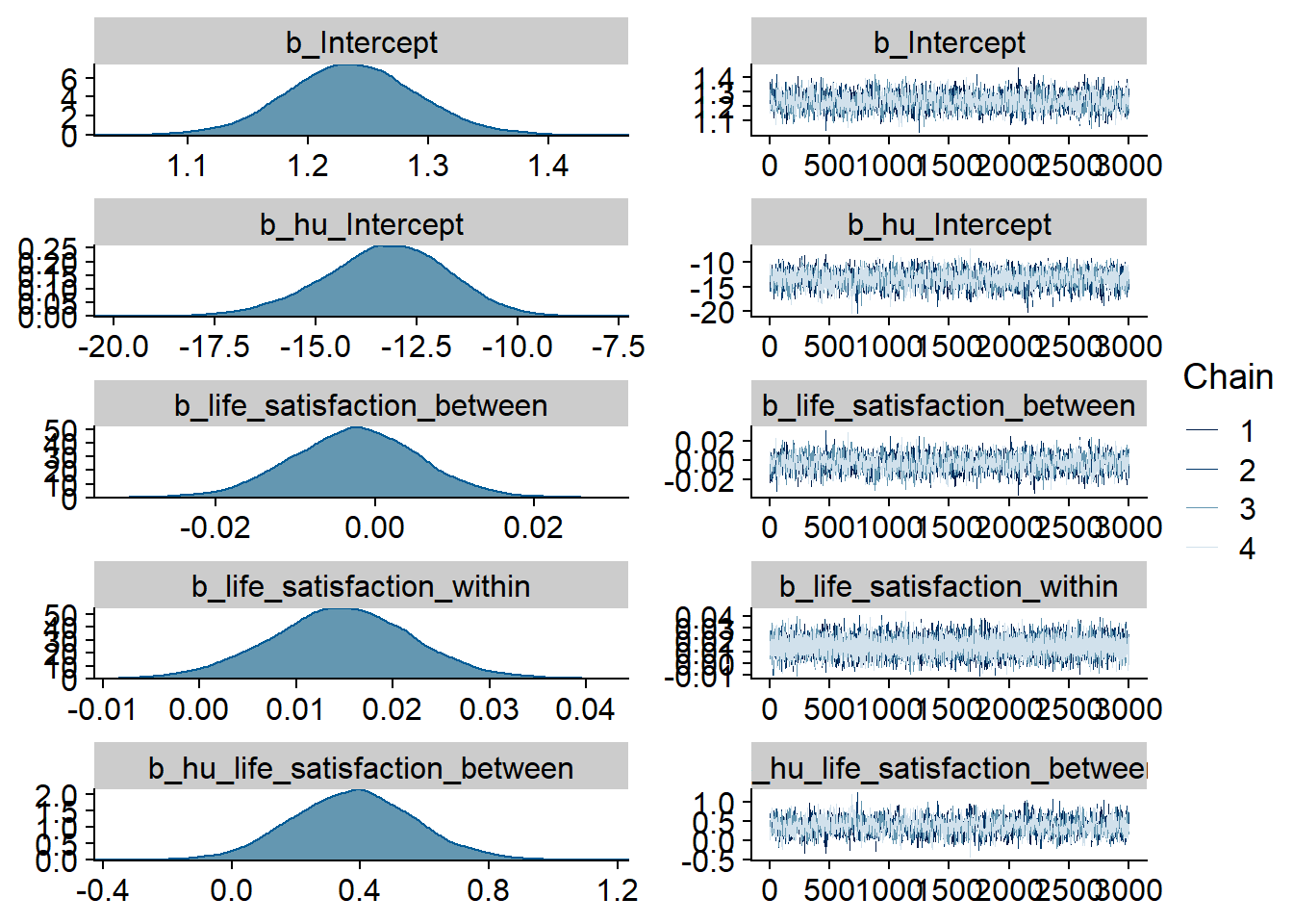
Figure 4.79: Traceplots and posterior distributions for Life Satisfaction-TV model
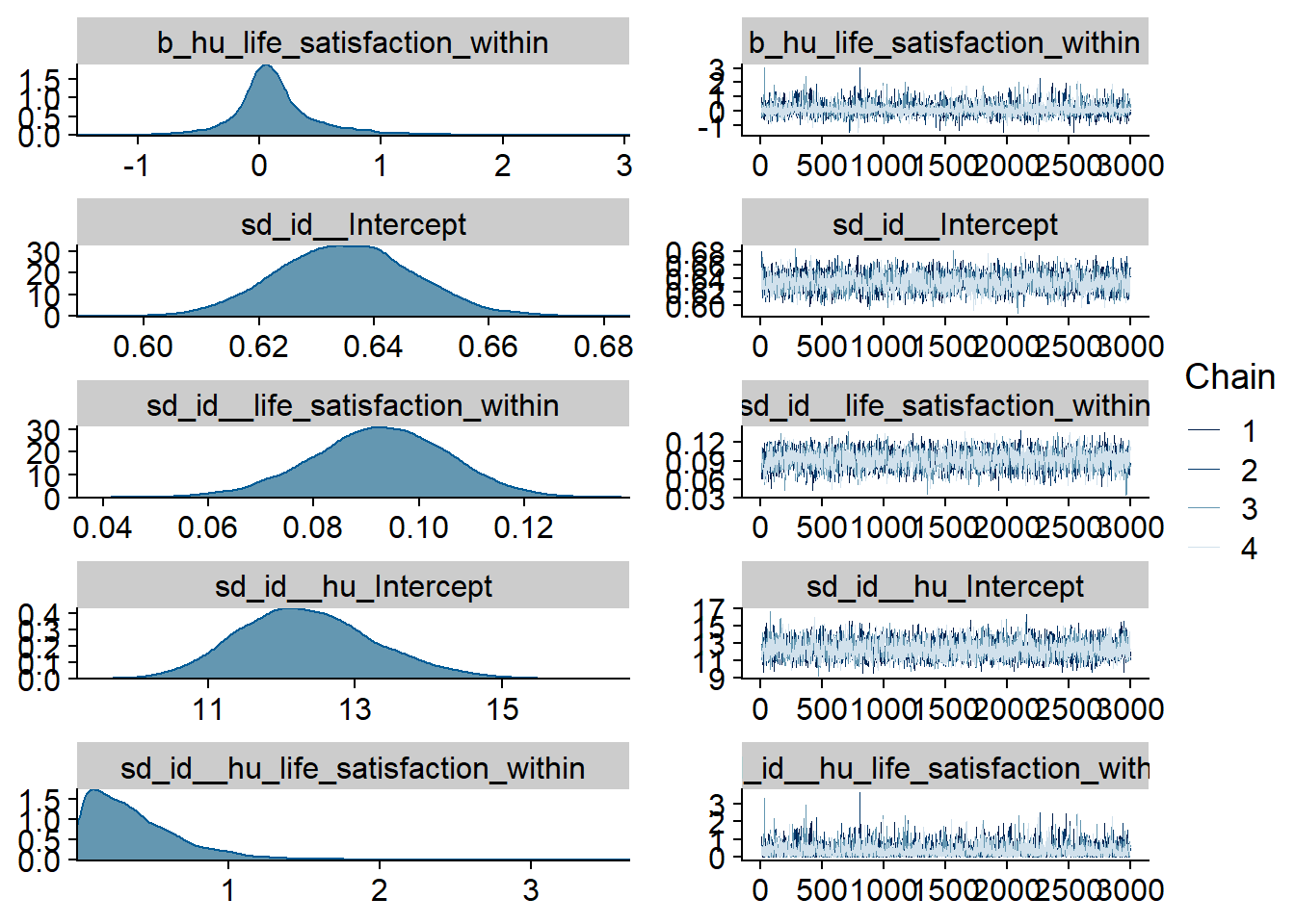
Figure 4.80: Traceplots and posterior distributions for Life Satisfaction-TV model
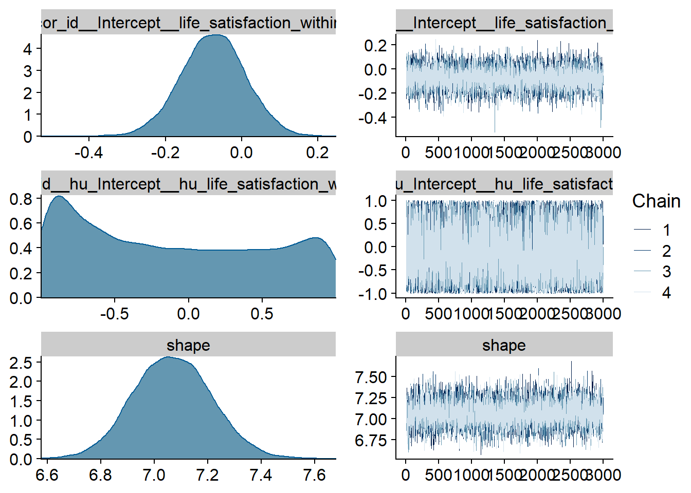
Figure 4.81: Traceplots and posterior distributions for Life Satisfaction-TV model
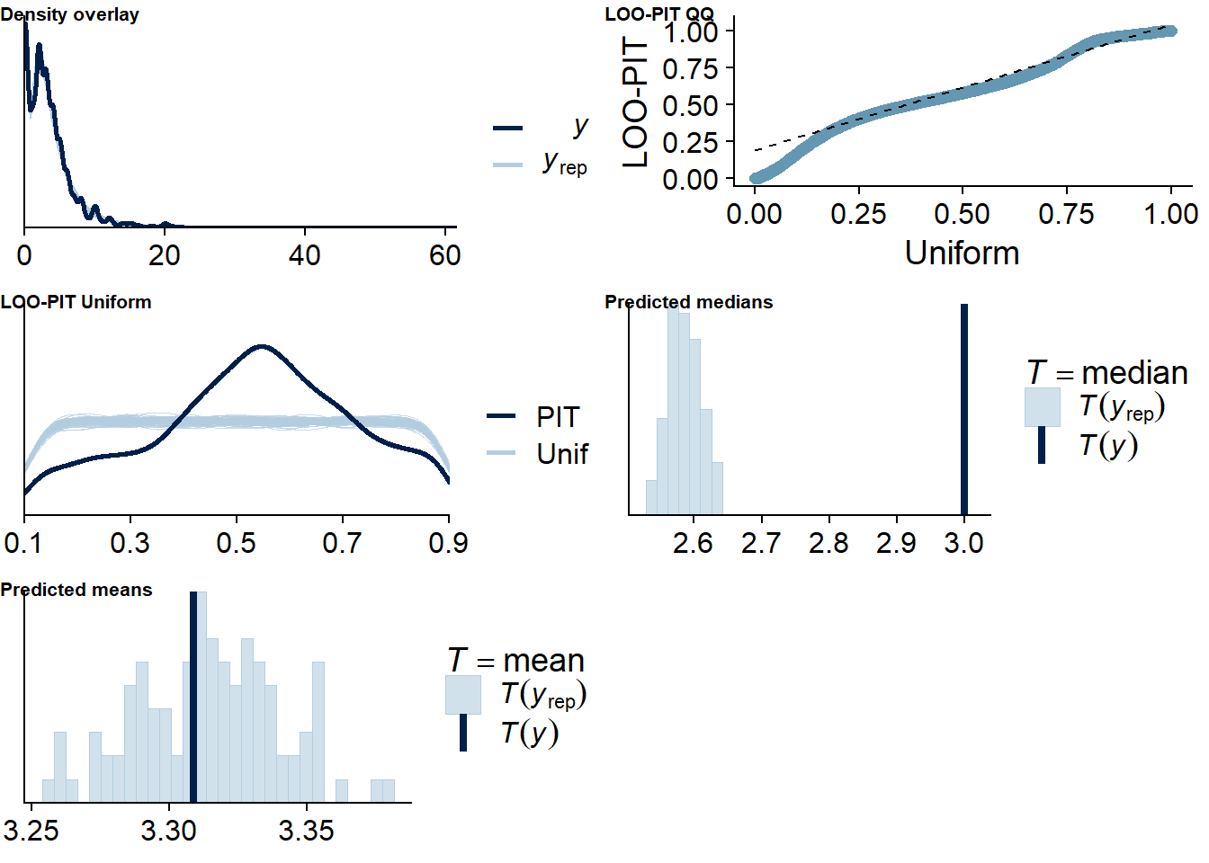
Figure 4.82: Posterior predictive checks for Life Satisfaction-TV model
The outliers are in about the same range as in previous models, and the model diagnostics look good.
life_tv_loo <- loo(life_tv)
life_tv_loo
##
## Computed from 12000 by 8698 log-likelihood matrix
##
## Estimate SE
## elpd_loo -13358.9 139.8
## p_loo 2078.6 56.1
## looic 26717.8 279.5
## ------
## Monte Carlo SE of elpd_loo is NA.
##
## Pareto k diagnostic values:
## Count Pct. Min. n_eff
## (-Inf, 0.5] (good) 7714 88.7% 833
## (0.5, 0.7] (ok) 623 7.2% 125
## (0.7, 1] (bad) 262 3.0% 16
## (1, Inf) (very bad) 99 1.1% 2
## See help('pareto-k-diagnostic') for details.Below the summary.
summary(life_tv)## Family: hurdle_gamma
## Links: mu = log; shape = identity; hu = logit
## Formula: lead_tv_time ~ 1 + life_satisfaction_between + life_satisfaction_within + (1 + life_satisfaction_within | id)
## hu ~ 1 + life_satisfaction_between + life_satisfaction_within + (1 + life_satisfaction_within | id)
## Data: working_file (Number of observations: 8698)
## Samples: 4 chains, each with iter = 5000; warmup = 2000; thin = 1;
## total post-warmup samples = 12000
##
## Group-Level Effects:
## ~id (Number of levels: 2157)
## Estimate Est.Error l-95% CI u-95% CI Rhat Bulk_ESS Tail_ESS
## sd(Intercept) 0.64 0.01 0.61 0.66 1.00 2373 4782
## sd(life_satisfaction_within) 0.09 0.01 0.07 0.12 1.00 2638 4171
## sd(hu_Intercept) 12.35 0.93 10.69 14.31 1.00 3129 6110
## sd(hu_life_satisfaction_within) 0.39 0.34 0.02 1.26 1.00 2890 4228
## cor(Intercept,life_satisfaction_within) -0.08 0.08 -0.24 0.09 1.00 12933 9443
## cor(hu_Intercept,hu_life_satisfaction_within) -0.12 0.64 -0.98 0.96 1.00 7309 6773
##
## Population-Level Effects:
## Estimate Est.Error l-95% CI u-95% CI Rhat Bulk_ESS Tail_ESS
## Intercept 1.24 0.05 1.13 1.34 1.00 1801 3195
## hu_Intercept -13.27 1.55 -16.45 -10.41 1.00 1938 3472
## life_satisfaction_between -0.00 0.01 -0.02 0.01 1.00 1878 3104
## life_satisfaction_within 0.01 0.01 0.00 0.03 1.00 16651 9659
## hu_life_satisfaction_between 0.38 0.19 0.01 0.76 1.00 1618 3056
## hu_life_satisfaction_within 0.13 0.36 -0.50 1.04 1.00 5016 4089
##
## Family Specific Parameters:
## Estimate Est.Error l-95% CI u-95% CI Rhat Bulk_ESS Tail_ESS
## shape 7.07 0.14 6.79 7.36 1.00 6724 9323
##
## Samples were drawn using sampling(NUTS). For each parameter, Bulk_ESS
## and Tail_ESS are effective sample size measures, and Rhat is the potential
## scale reduction factor on split chains (at convergence, Rhat = 1).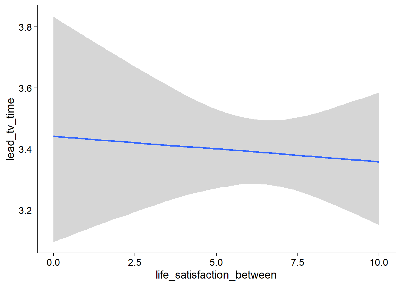
Figure 4.83: Conditional effects for Life Satisfaction-TV model
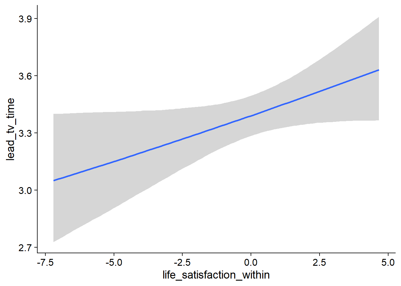
Figure 4.84: Conditional effects for Life Satisfaction-TV model
4.5 Video games
4.5.1 Affect
4.5.1.1 Games on affect
games_affect <-
  brm(
    data = working_file,
    family = gaussian,
    affect ~
      1 +
      games_used_between +
      games_used_within +
      games_time_between +
      games_time_within +
      (1 +
         games_time_within +
         games_used_within
       | id),
    iter = 5000,
    warmup = 2000,
    chains = 4,
    cores = 4,
    seed = 42,
    control = list(adapt_delta = 0.95),
    file = here("models", "games_affect")
  )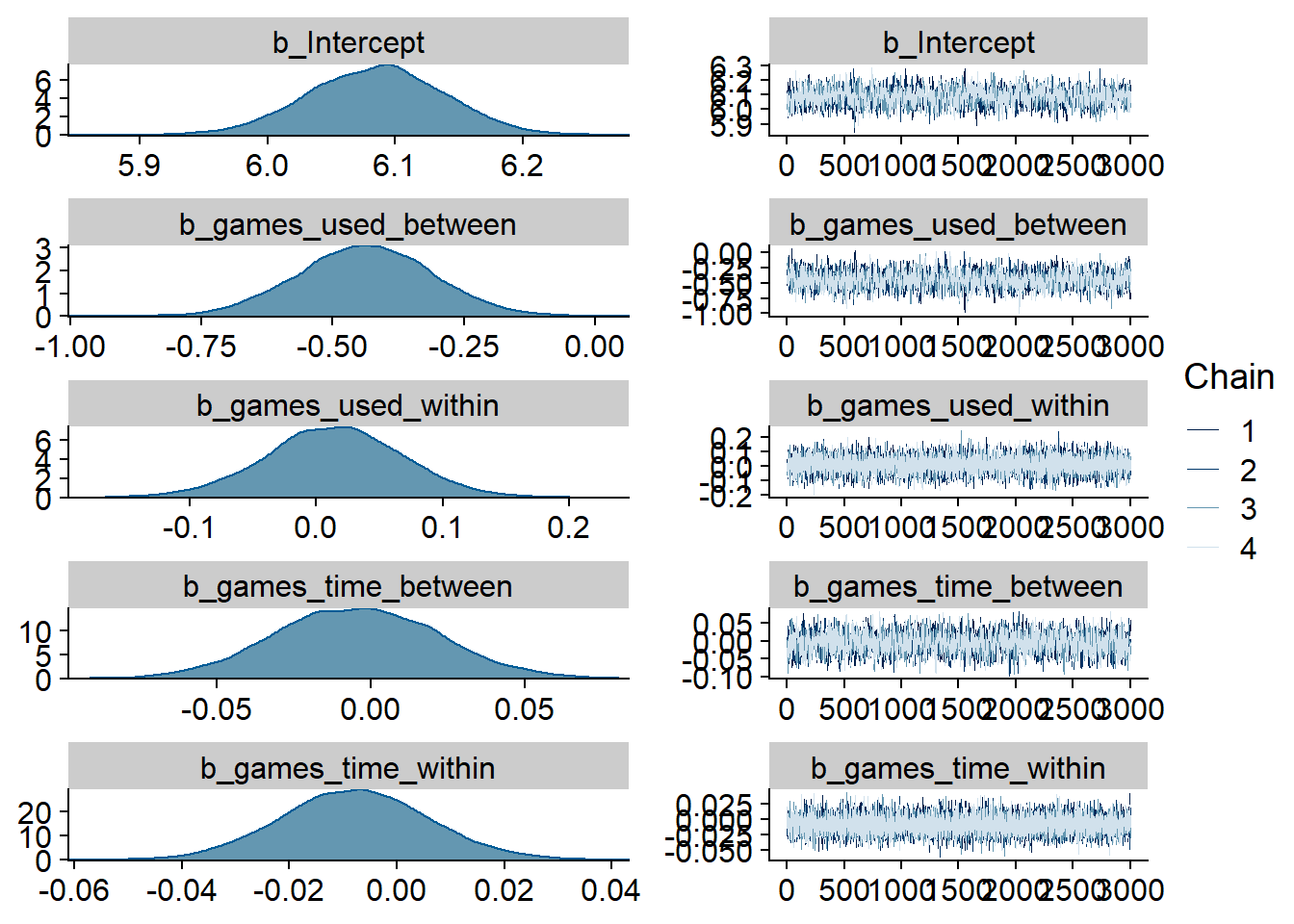
Figure 4.85: Traceplots and posterior distributions for Games-Affect model
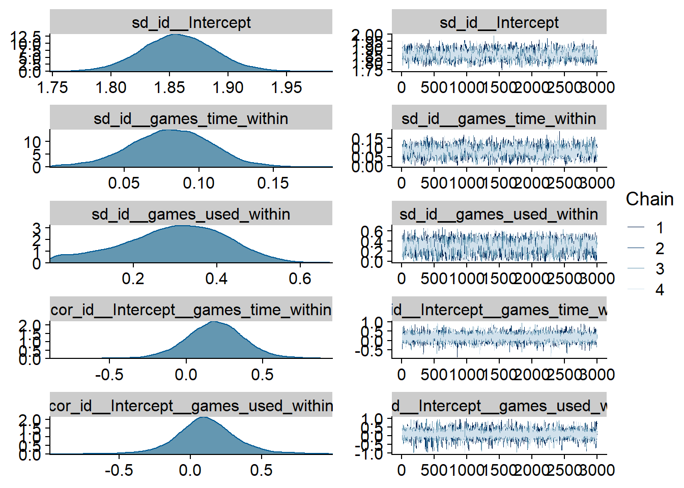
Figure 4.86: Traceplots and posterior distributions for Games-Affect model
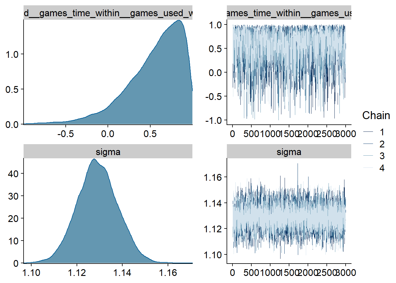
Figure 4.87: Traceplots and posterior distributions for Games-Affect model
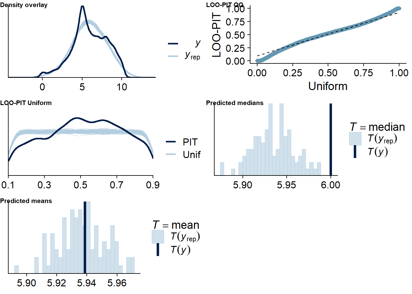
Figure 4.88: Posterior predictive checks for Games-Affect model
The outliers are in about the same range as in previous models, and the model diagnostics look good.
games_affect_loo <- loo(games_affect)
games_affect_loo
##
## Computed from 12000 by 10985 log-likelihood matrix
##
## Estimate SE
## elpd_loo -18108.9 105.5
## p_loo 1992.1 34.8
## looic 36217.9 210.9
## ------
## Monte Carlo SE of elpd_loo is NA.
##
## Pareto k diagnostic values:
## Count Pct. Min. n_eff
## (-Inf, 0.5] (good) 10558 96.1% 554
## (0.5, 0.7] (ok) 378 3.4% 114
## (0.7, 1] (bad) 49 0.4% 16
## (1, Inf) (very bad) 0 0.0% <NA>
## See help('pareto-k-diagnostic') for details.Below the summary.
summary(games_affect)## Family: gaussian
## Links: mu = identity; sigma = identity
## Formula: affect ~ 1 + games_used_between + games_used_within + games_time_between + games_time_within + (1 + games_time_within + games_used_within | id)
## Data: working_file (Number of observations: 10985)
## Samples: 4 chains, each with iter = 5000; warmup = 2000; thin = 1;
## total post-warmup samples = 12000
##
## Group-Level Effects:
## ~id (Number of levels: 2159)
## Estimate Est.Error l-95% CI u-95% CI Rhat Bulk_ESS Tail_ESS
## sd(Intercept) 1.86 0.03 1.80 1.92 1.00 2195 4042
## sd(games_time_within) 0.08 0.03 0.02 0.13 1.00 1895 2608
## sd(games_used_within) 0.30 0.12 0.03 0.52 1.00 1818 2315
## cor(Intercept,games_time_within) 0.19 0.19 -0.20 0.57 1.00 10965 6328
## cor(Intercept,games_used_within) 0.11 0.23 -0.36 0.60 1.00 9623 4545
## cor(games_time_within,games_used_within) 0.55 0.33 -0.26 0.96 1.00 2411 3963
##
## Population-Level Effects:
## Estimate Est.Error l-95% CI u-95% CI Rhat Bulk_ESS Tail_ESS
## Intercept 6.08 0.05 5.98 6.19 1.00 1676 3086
## games_used_between -0.44 0.13 -0.69 -0.19 1.00 1757 3418
## games_used_within 0.01 0.05 -0.09 0.12 1.00 22134 8654
## games_time_between -0.00 0.03 -0.06 0.05 1.00 2177 4108
## games_time_within -0.01 0.01 -0.03 0.02 1.00 15696 10619
##
## Family Specific Parameters:
## Estimate Est.Error l-95% CI u-95% CI Rhat Bulk_ESS Tail_ESS
## sigma 1.13 0.01 1.11 1.15 1.00 8760 9049
##
## Samples were drawn using sampling(NUTS). For each parameter, Bulk_ESS
## and Tail_ESS are effective sample size measures, and Rhat is the potential
## scale reduction factor on split chains (at convergence, Rhat = 1).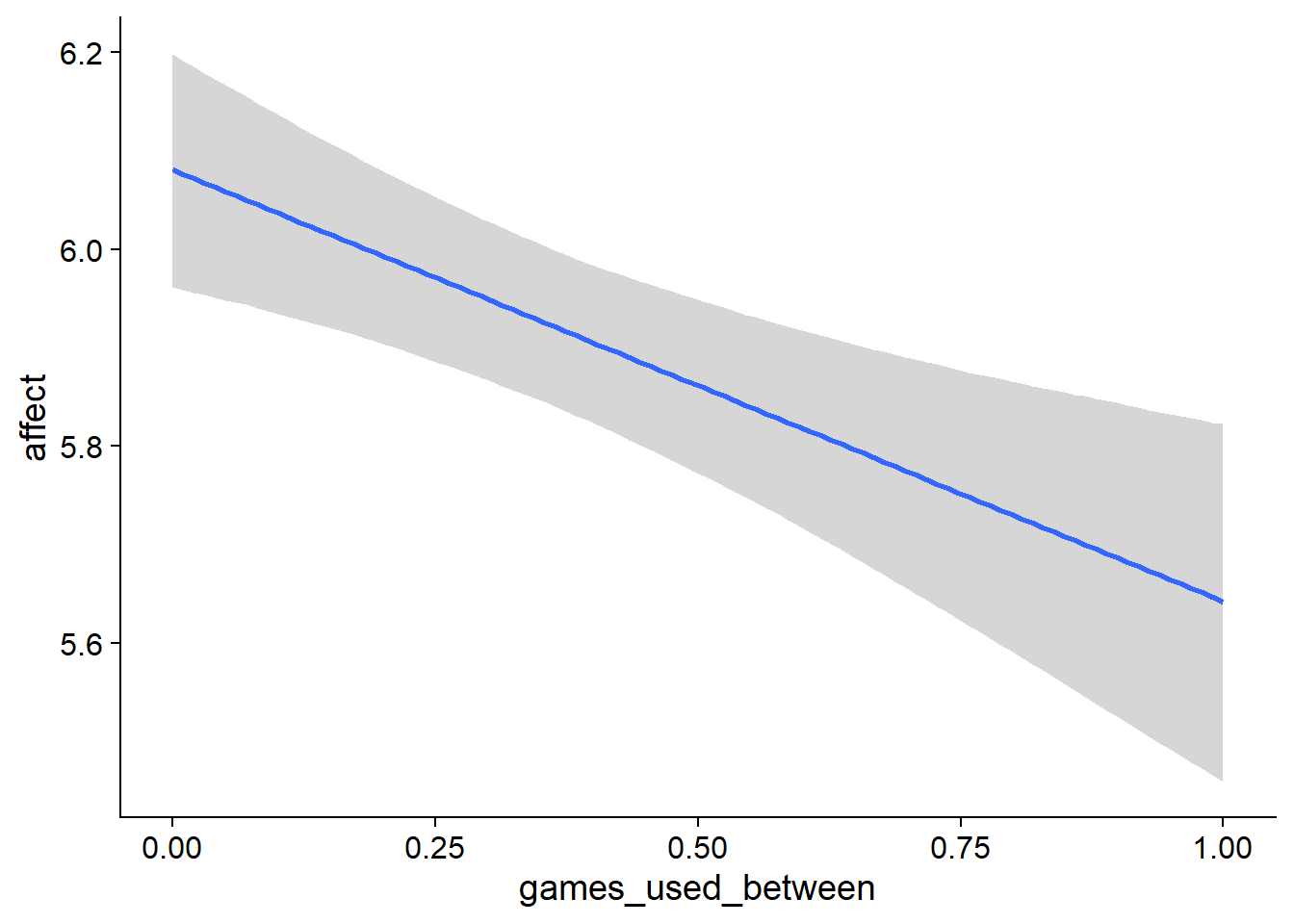
Figure 4.89: Conditional effects for Games-Affect model
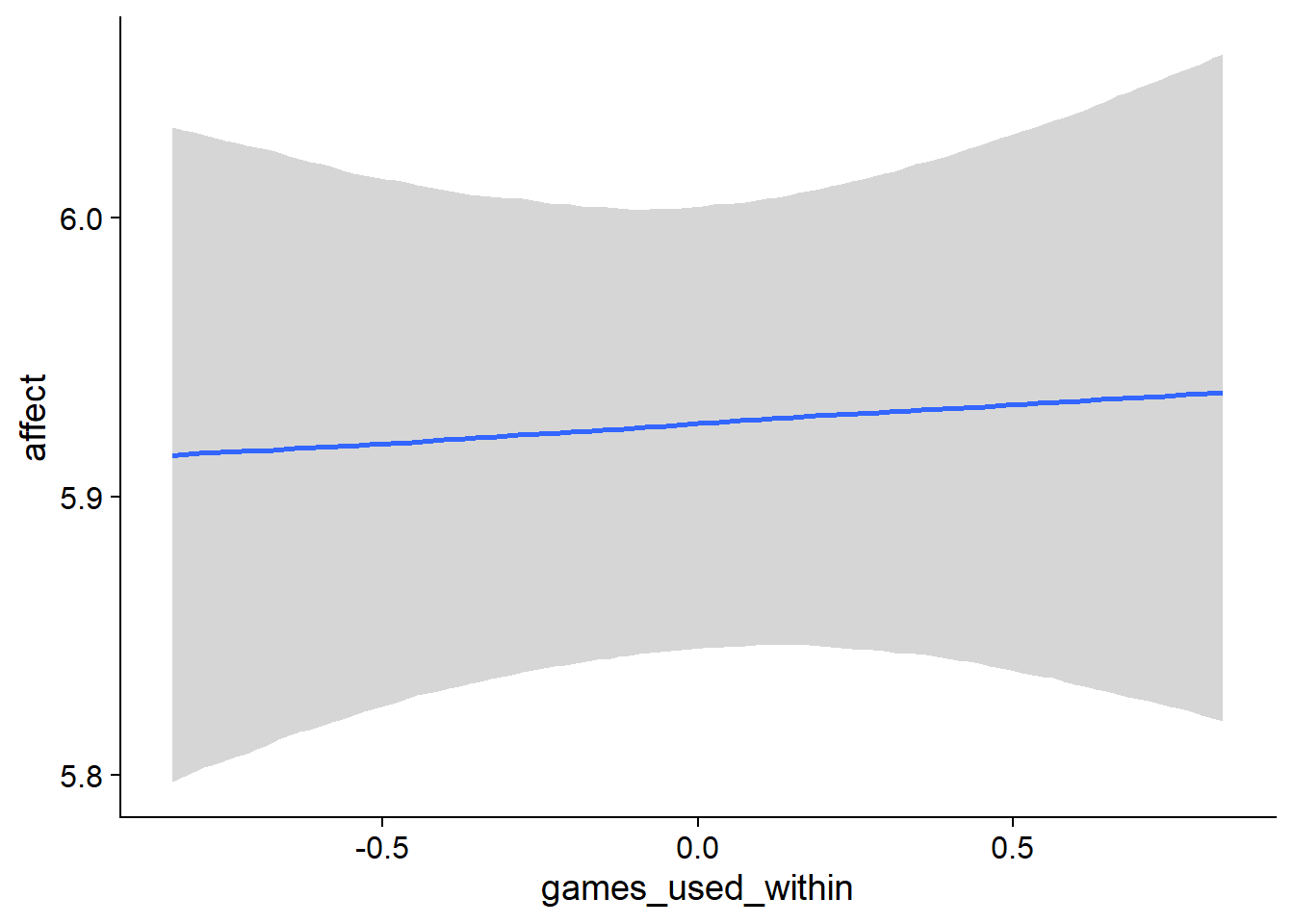
Figure 4.90: Conditional effects for Games-Affect model
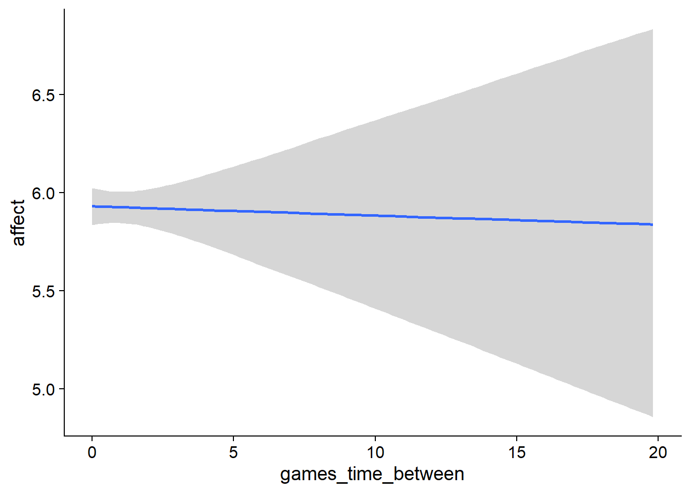
Figure 4.91: Conditional effects for Games-Affect model
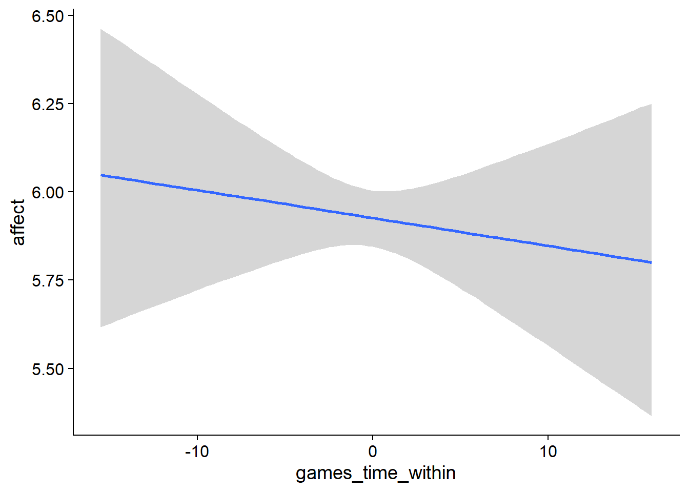
Figure 4.92: Conditional effects for Games-Affect model
##            used  (Mb) gc trigger   (Mb)  max used   (Mb)
## Ncells  3692797 197.3    6044351  322.9   6044351  322.9
## Vcells 23776926 181.5  148227097 1130.9 231600594 1767.0
4.5.1.2 Affect on video games
affect_games <-
  brm(
    bf(
      # predicting continuous part
      lead_games_time ~
        1 +
        affect_between +
        affect_within +
        (1 +
           affect_within
         | id),

      # predicting hurdle part
      hu ~
        1 +
        affect_between +
        affect_within +
        (1 +
           affect_within
         | id)
    ),
    data = working_file,
    family = hurdle_gamma(),
    ,
    iter = 5000,
    warmup = 2000,
    chains = 4,
    cores = 4,
    seed = 42,
    control = list(adapt_delta = 0.95),
    file = here("models", "affect_games")
  )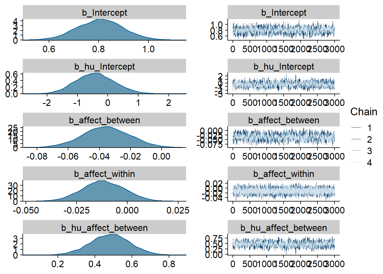
Figure 4.93: Traceplots and posterior distributions for Affect-Games model
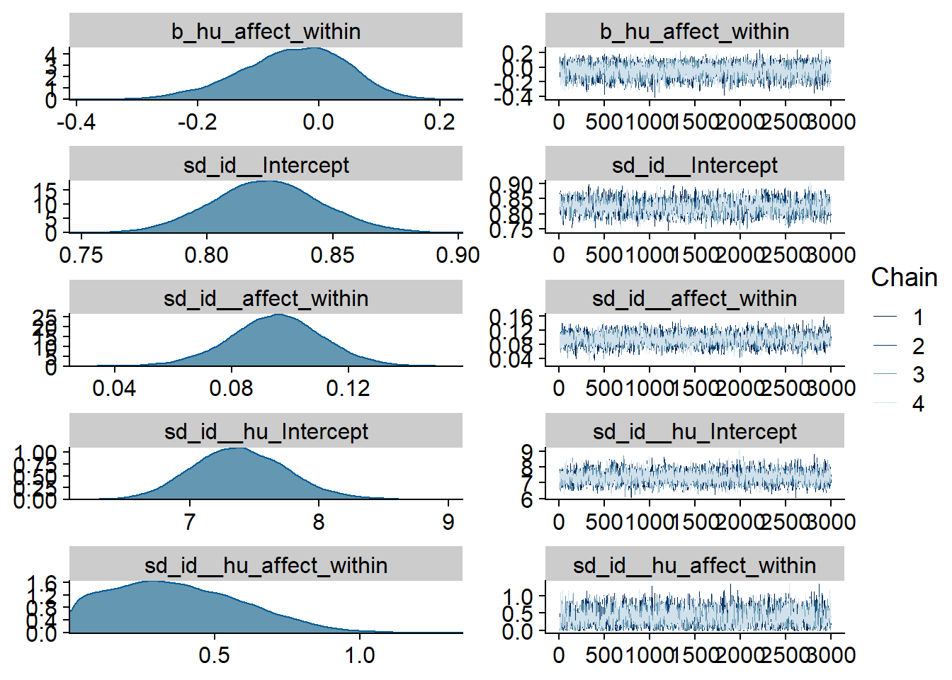
Figure 4.94: Traceplots and posterior distributions for Affect-Games model
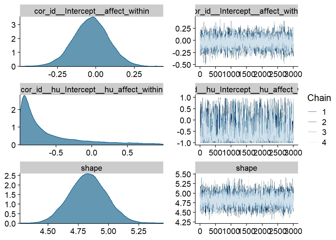
Figure 4.95: Traceplots and posterior distributions for Affect-Games model
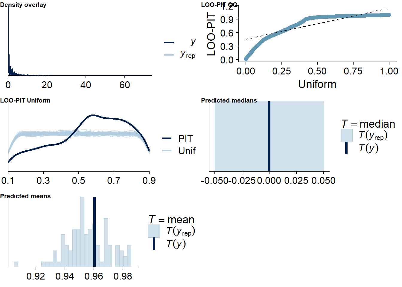
Figure 4.96: Posterior predictive checks for Affect-Games model
There are more potentially influential values than in previous models.
affect_games_loo <- loo(affect_games)
affect_games_loo
##
## Computed from 12000 by 8698 log-likelihood matrix
##
## Estimate SE
## elpd_loo -6436.2 113.9
## p_loo 1729.1 46.5
## looic 12872.5 227.8
## ------
## Monte Carlo SE of elpd_loo is NA.
##
## Pareto k diagnostic values:
## Count Pct. Min. n_eff
## (-Inf, 0.5] (good) 7565 87.0% 803
## (0.5, 0.7] (ok) 682 7.8% 154
## (0.7, 1] (bad) 364 4.2% 17
## (1, Inf) (very bad) 87 1.0% 4
## See help('pareto-k-diagnostic') for details.Below the summary.
summary(affect_games)## Family: hurdle_gamma
## Links: mu = log; shape = identity; hu = logit
## Formula: lead_games_time ~ 1 + affect_between + affect_within + (1 + affect_within | id)
## hu ~ 1 + affect_between + affect_within + (1 + affect_within | id)
## Data: working_file (Number of observations: 8698)
## Samples: 4 chains, each with iter = 5000; warmup = 2000; thin = 1;
## total post-warmup samples = 12000
##
## Group-Level Effects:
## ~id (Number of levels: 2157)
## Estimate Est.Error l-95% CI u-95% CI Rhat Bulk_ESS Tail_ESS
## sd(Intercept) 0.82 0.02 0.78 0.87 1.00 1638 3514
## sd(affect_within) 0.10 0.02 0.06 0.13 1.00 2274 3040
## sd(hu_Intercept) 7.39 0.36 6.71 8.14 1.00 2528 4976
## sd(hu_affect_within) 0.37 0.23 0.02 0.85 1.00 1483 2155
## cor(Intercept,affect_within) -0.03 0.12 -0.26 0.19 1.00 7302 7705
## cor(hu_Intercept,hu_affect_within) -0.63 0.43 -0.99 0.63 1.00 2975 4946
##
## Population-Level Effects:
## Estimate Est.Error l-95% CI u-95% CI Rhat Bulk_ESS Tail_ESS
## Intercept 0.80 0.09 0.62 0.98 1.01 1060 2620
## hu_Intercept -0.42 0.63 -1.63 0.85 1.01 963 2042
## affect_between -0.04 0.02 -0.07 -0.01 1.00 1043 2736
## affect_within -0.01 0.01 -0.03 0.01 1.00 8115 8815
## hu_affect_between 0.48 0.11 0.27 0.69 1.01 957 2069
## hu_affect_within -0.04 0.09 -0.22 0.11 1.00 3045 6968
##
## Family Specific Parameters:
## Estimate Est.Error l-95% CI u-95% CI Rhat Bulk_ESS Tail_ESS
## shape 4.83 0.15 4.53 5.13 1.00 4742 6948
##
## Samples were drawn using sampling(NUTS). For each parameter, Bulk_ESS
## and Tail_ESS are effective sample size measures, and Rhat is the potential
## scale reduction factor on split chains (at convergence, Rhat = 1).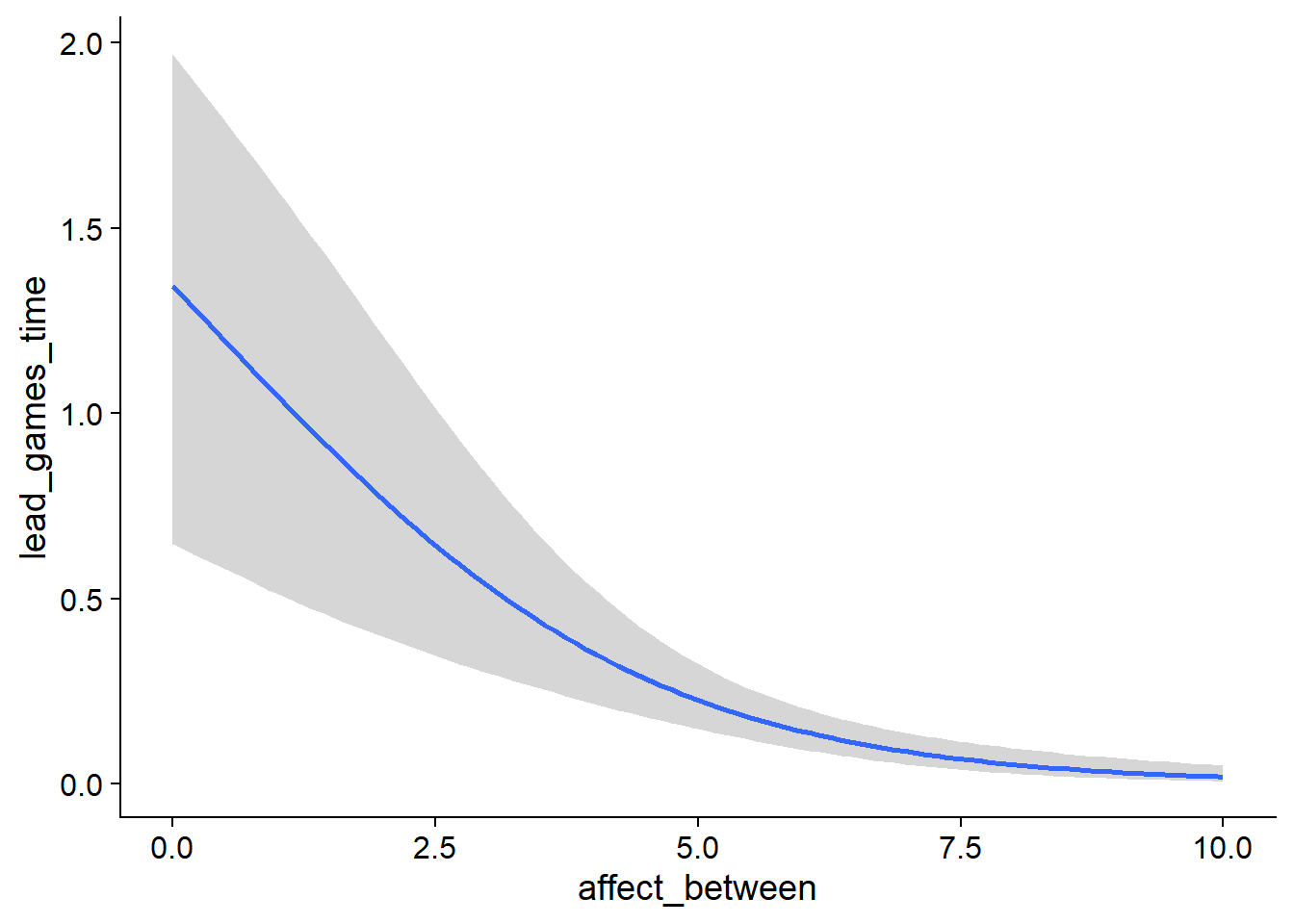
Figure 4.97: Conditional effects for Affect-Games model
Figure 4.98: Conditional effects for Affect-Games model
##            used  (Mb) gc trigger   (Mb)  max used   (Mb)
## Ncells  3692873 197.3    6044351  322.9   6044351  322.9
## Vcells 23777835 181.5  174444794 1331.0 231600594 1767.0
4.5.2 Life satisfaction
4.5.2.1 Games on life satisfaction
The correlation between random effects has quite few samples, which is why I had to increase the interations.
games_life <-
  brm(
    data = working_file,
    family = gaussian,
    life_satisfaction ~
      1 +
      games_used_between +
      games_used_within +
      games_time_between +
      games_time_within +
      (1 +
         games_time_within +
         games_used_within
       | id),
    iter = 8000,
    warmup = 3000,
    chains = 4,
    cores = 4,
    seed = 42,
    control = list(adapt_delta = 0.95),
    file = here("models", "games_life")
  )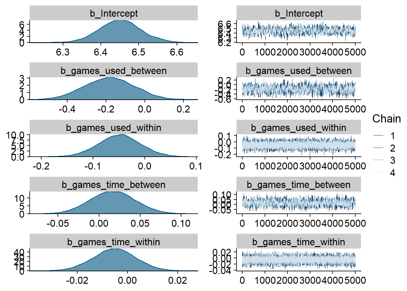
Figure 4.99: Traceplots and posterior distributions for Games-Life Satisfaction model
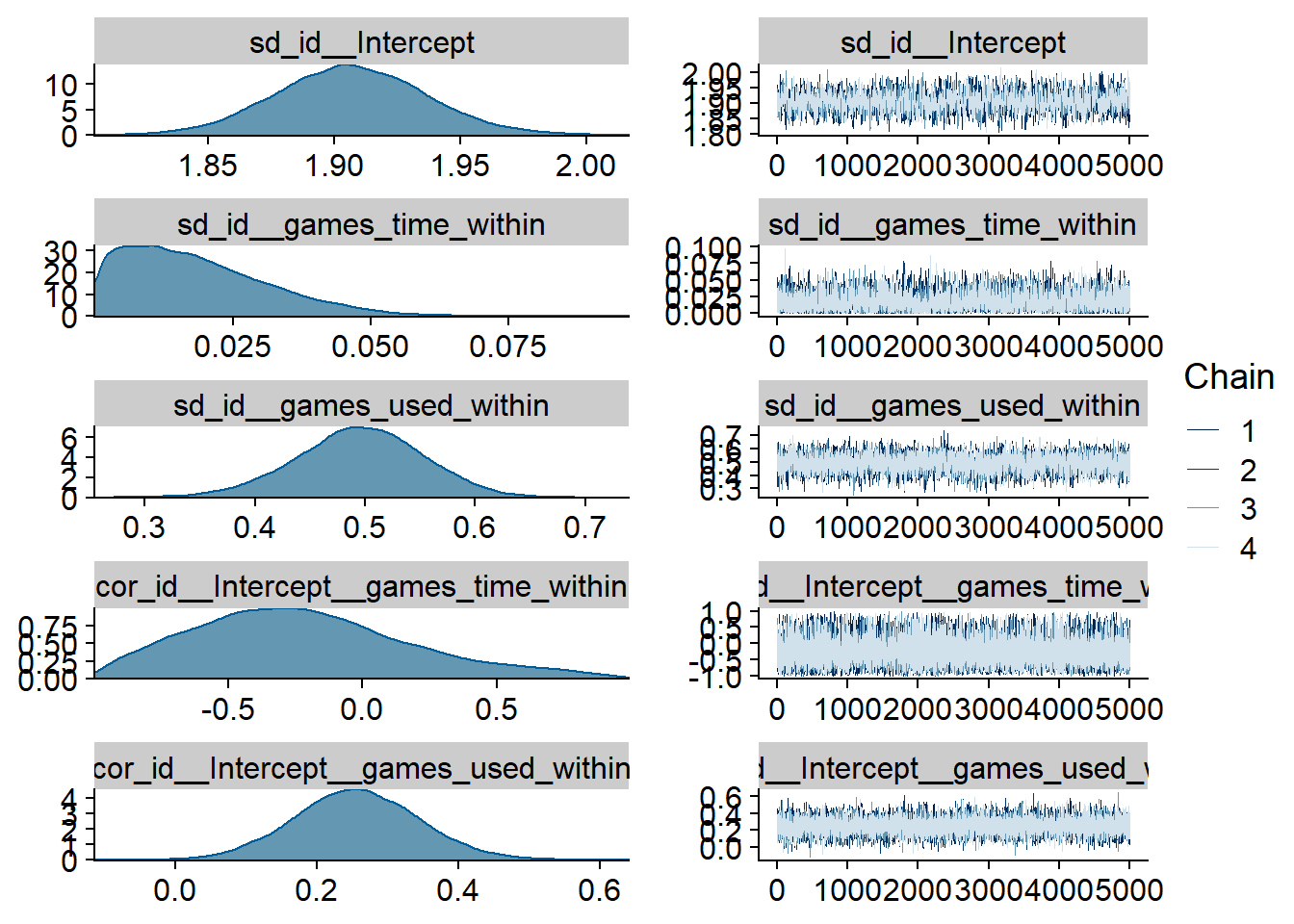
Figure 4.100: Traceplots and posterior distributions for Games-Life Satisfaction model
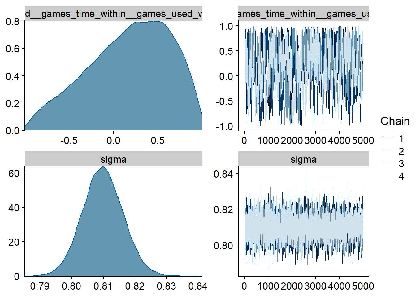
Figure 4.101: Traceplots and posterior distributions for Games-Life Satisfaction model
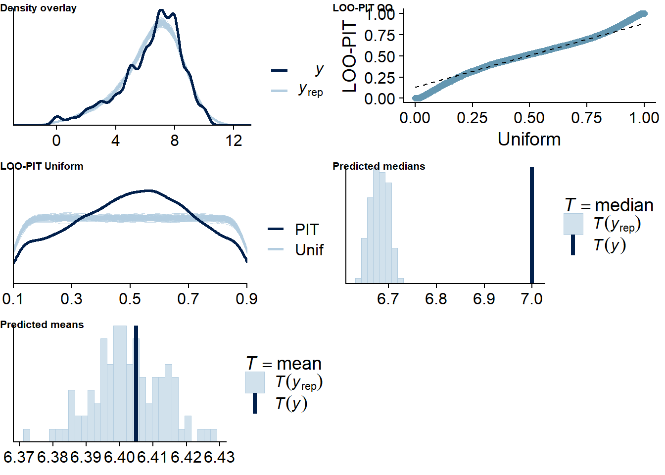
Figure 4.102: Posterior predictive checks for Games-Life Satisfaction model
The outliers are in about the same range as in previous models, and the model diagnostics look good.
games_life_loo <- loo(games_life)
games_life_loo
##
## Computed from 20000 by 10985 log-likelihood matrix
##
## Estimate SE
## elpd_loo -14565.9 143.4
## p_loo 2144.5 51.4
## looic 29131.9 286.9
## ------
## Monte Carlo SE of elpd_loo is NA.
##
## Pareto k diagnostic values:
## Count Pct. Min. n_eff
## (-Inf, 0.5] (good) 10500 95.6% 736
## (0.5, 0.7] (ok) 404 3.7% 132
## (0.7, 1] (bad) 73 0.7% 19
## (1, Inf) (very bad) 8 0.1% 3
## See help('pareto-k-diagnostic') for details.Below the summary.
summary(games_life)## Family: gaussian
## Links: mu = identity; sigma = identity
## Formula: life_satisfaction ~ 1 + games_used_between + games_used_within + games_time_between + games_time_within + (1 + games_time_within + games_used_within | id)
## Data: working_file (Number of observations: 10985)
## Samples: 4 chains, each with iter = 8000; warmup = 3000; thin = 1;
## total post-warmup samples = 20000
##
## Group-Level Effects:
## ~id (Number of levels: 2159)
## Estimate Est.Error l-95% CI u-95% CI Rhat Bulk_ESS Tail_ESS
## sd(Intercept) 1.91 0.03 1.85 1.97 1.00 1728 3684
## sd(games_time_within) 0.02 0.01 0.00 0.05 1.00 1681 5445
## sd(games_used_within) 0.49 0.06 0.38 0.60 1.00 3174 8897
## cor(Intercept,games_time_within) -0.22 0.40 -0.89 0.69 1.00 19642 12094
## cor(Intercept,games_used_within) 0.26 0.09 0.08 0.43 1.00 10286 11790
## cor(games_time_within,games_used_within) 0.17 0.46 -0.78 0.89 1.01 313 517
##
## Population-Level Effects:
## Estimate Est.Error l-95% CI u-95% CI Rhat Bulk_ESS Tail_ESS
## Intercept 6.45 0.05 6.34 6.56 1.01 813 1730
## games_used_between -0.18 0.13 -0.43 0.07 1.00 1064 2301
## games_used_within -0.05 0.04 -0.13 0.03 1.00 23383 17438
## games_time_between 0.02 0.03 -0.04 0.07 1.00 1294 2646
## games_time_within -0.01 0.01 -0.02 0.01 1.00 26625 16601
##
## Family Specific Parameters:
## Estimate Est.Error l-95% CI u-95% CI Rhat Bulk_ESS Tail_ESS
## sigma 0.81 0.01 0.80 0.82 1.00 17578 15429
##
## Samples were drawn using sampling(NUTS). For each parameter, Bulk_ESS
## and Tail_ESS are effective sample size measures, and Rhat is the potential
## scale reduction factor on split chains (at convergence, Rhat = 1).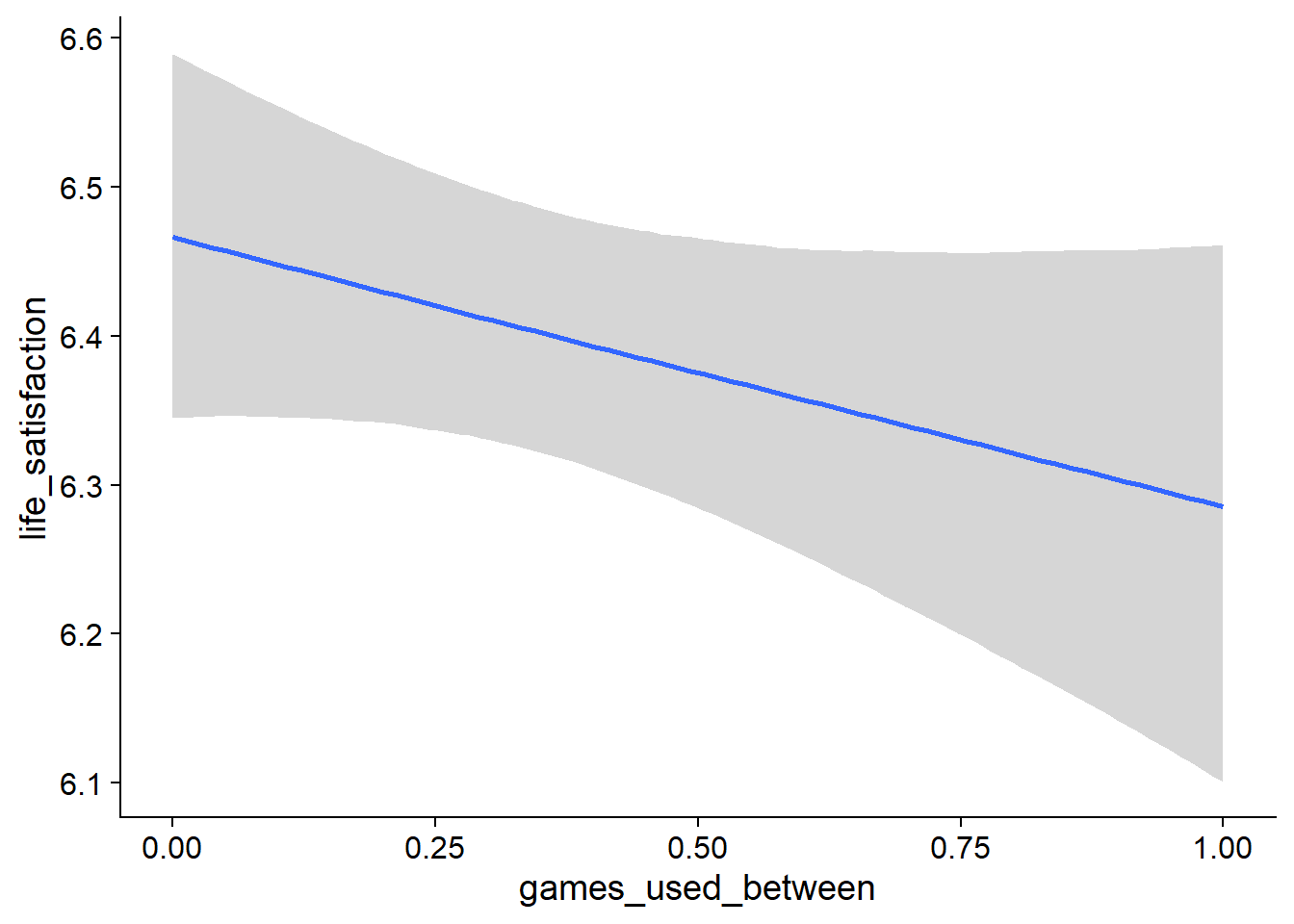
Figure 4.103: Conditional effects for Games-Life Satisfaction model
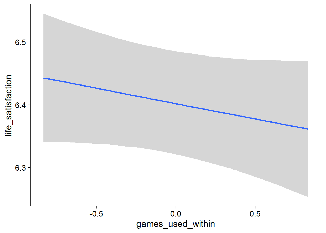
Figure 4.104: Conditional effects for Games-Life Satisfaction model
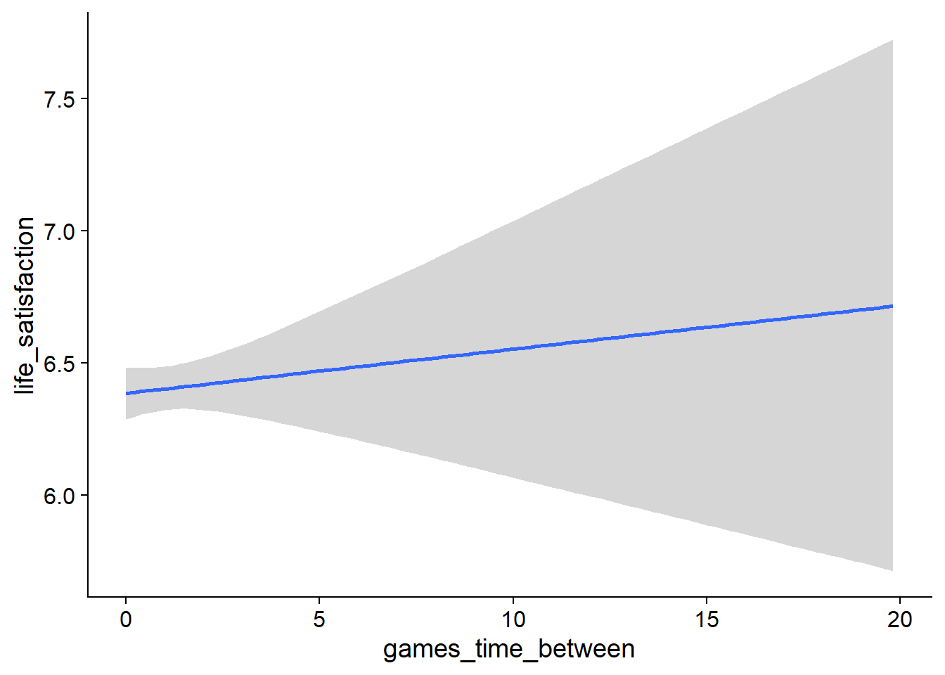
Figure 4.105: Conditional effects for Games-Life Satisfaction model
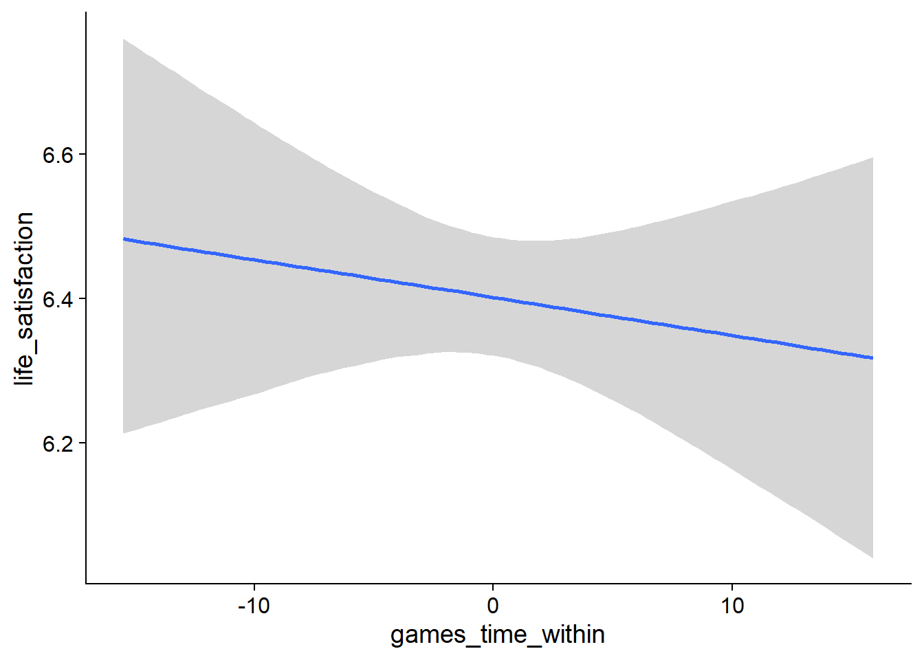
Figure 4.106: Conditional effects for Games-Life Satisfaction model
##            used  (Mb) gc trigger   (Mb)  max used   (Mb)
## Ncells  3692973 197.3    6044351  322.9   6044351  322.9
## Vcells 23778825 181.5  204656268 1561.5 255811179 1951.7
4.5.2.2 Life satisfaction on video games
life_games <-
  brm(
    bf(
      # predicting continuous part
      lead_games_time ~
        1 +
        life_satisfaction_between +
        life_satisfaction_within +
        (1 +
           life_satisfaction_within
         | id),

      # predicting hurdle part
      hu ~
        1 +
        life_satisfaction_between +
        life_satisfaction_within +
        (1 +
           life_satisfaction_within
         | id)
    ),
    data = working_file,
    family = hurdle_gamma(),
    ,
    iter = 5000,
    warmup = 2000,
    chains = 4,
    cores = 4,
    seed = 42,
    control = list(adapt_delta = 0.95),
    file = here("models", "life_games")
  )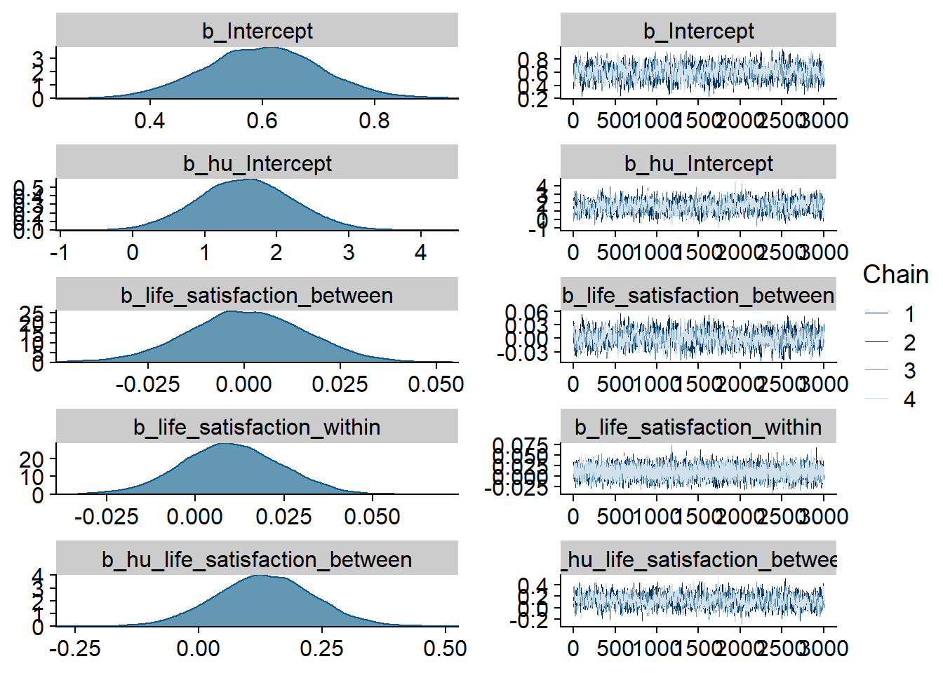
Figure 4.107: Traceplots and posterior distributions for Life Satisfaction-Games model
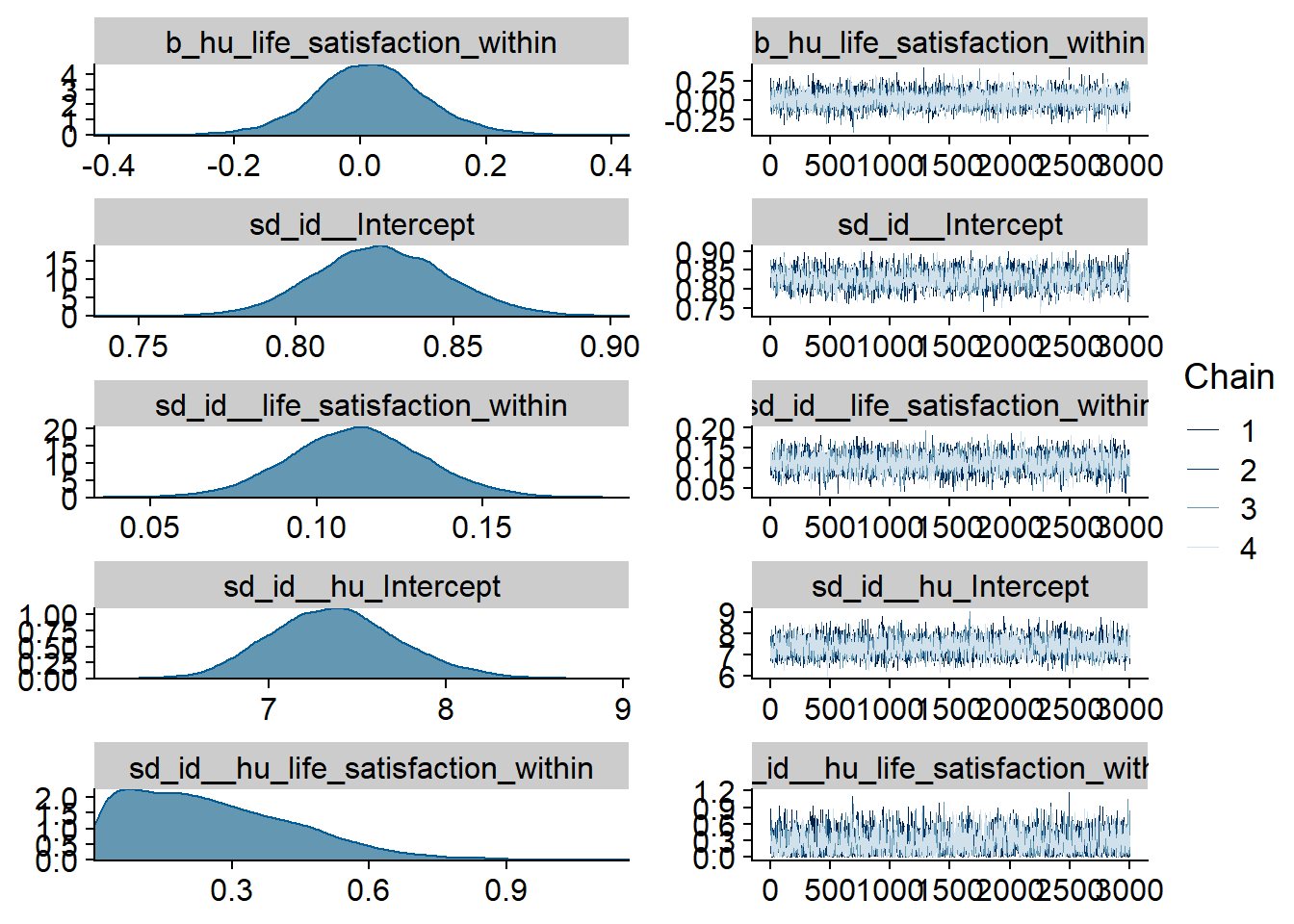
Figure 4.108: Traceplots and posterior distributions for Life Satisfaction-Games model
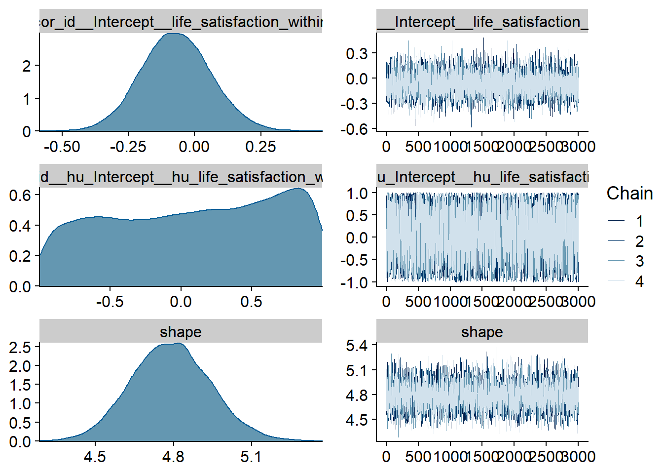
Figure 4.109: Traceplots and posterior distributions for Life Satisfaction-Games model
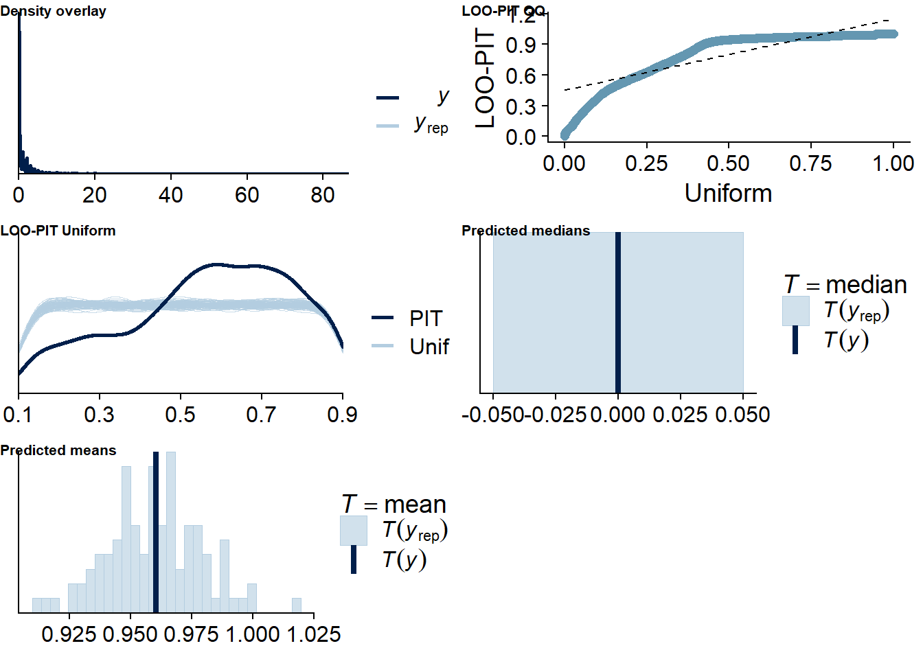
Figure 4.110: Posterior predictive checks for Life Satisfaction-Games model
There are more potentially influential values than in previous models.
life_games_loo <- loo(life_games)
life_games_loo
##
## Computed from 12000 by 8698 log-likelihood matrix
##
## Estimate SE
## elpd_loo -6444.4 114.7
## p_loo 1711.5 47.0
## looic 12888.9 229.4
## ------
## Monte Carlo SE of elpd_loo is NA.
##
## Pareto k diagnostic values:
## Count Pct. Min. n_eff
## (-Inf, 0.5] (good) 7645 87.9% 773
## (0.5, 0.7] (ok) 635 7.3% 153
## (0.7, 1] (bad) 337 3.9% 20
## (1, Inf) (very bad) 81 0.9% 2
## See help('pareto-k-diagnostic') for details.Below the summary.
summary(life_games)## Family: hurdle_gamma
## Links: mu = log; shape = identity; hu = logit
## Formula: lead_games_time ~ 1 + life_satisfaction_between + life_satisfaction_within + (1 + life_satisfaction_within | id)
## hu ~ 1 + life_satisfaction_between + life_satisfaction_within + (1 + life_satisfaction_within | id)
## Data: working_file (Number of observations: 8698)
## Samples: 4 chains, each with iter = 5000; warmup = 2000; thin = 1;
## total post-warmup samples = 12000
##
## Group-Level Effects:
## ~id (Number of levels: 2157)
## Estimate Est.Error l-95% CI u-95% CI Rhat Bulk_ESS Tail_ESS
## sd(Intercept) 0.83 0.02 0.79 0.87 1.00 1914 4056
## sd(life_satisfaction_within) 0.11 0.02 0.07 0.15 1.00 3140 4693
## sd(hu_Intercept) 7.38 0.37 6.71 8.14 1.00 2956 5758
## sd(hu_life_satisfaction_within) 0.26 0.18 0.01 0.66 1.00 2015 3886
## cor(Intercept,life_satisfaction_within) -0.07 0.13 -0.32 0.19 1.00 8424 8566
## cor(hu_Intercept,hu_life_satisfaction_within) 0.09 0.59 -0.93 0.97 1.00 6667 6234
##
## Population-Level Effects:
## Estimate Est.Error l-95% CI u-95% CI Rhat Bulk_ESS Tail_ESS
## Intercept 0.60 0.10 0.40 0.80 1.00 1160 2193
## hu_Intercept 1.56 0.66 0.28 2.87 1.00 1407 2638
## life_satisfaction_between 0.00 0.02 -0.03 0.03 1.00 1184 2259
## life_satisfaction_within 0.01 0.01 -0.02 0.04 1.00 8793 9142
## hu_life_satisfaction_between 0.13 0.10 -0.06 0.33 1.00 1323 2507
## hu_life_satisfaction_within 0.02 0.09 -0.16 0.20 1.00 8294 6754
##
## Family Specific Parameters:
## Estimate Est.Error l-95% CI u-95% CI Rhat Bulk_ESS Tail_ESS
## shape 4.79 0.15 4.50 5.09 1.00 6117 8149
##
## Samples were drawn using sampling(NUTS). For each parameter, Bulk_ESS
## and Tail_ESS are effective sample size measures, and Rhat is the potential
## scale reduction factor on split chains (at convergence, Rhat = 1).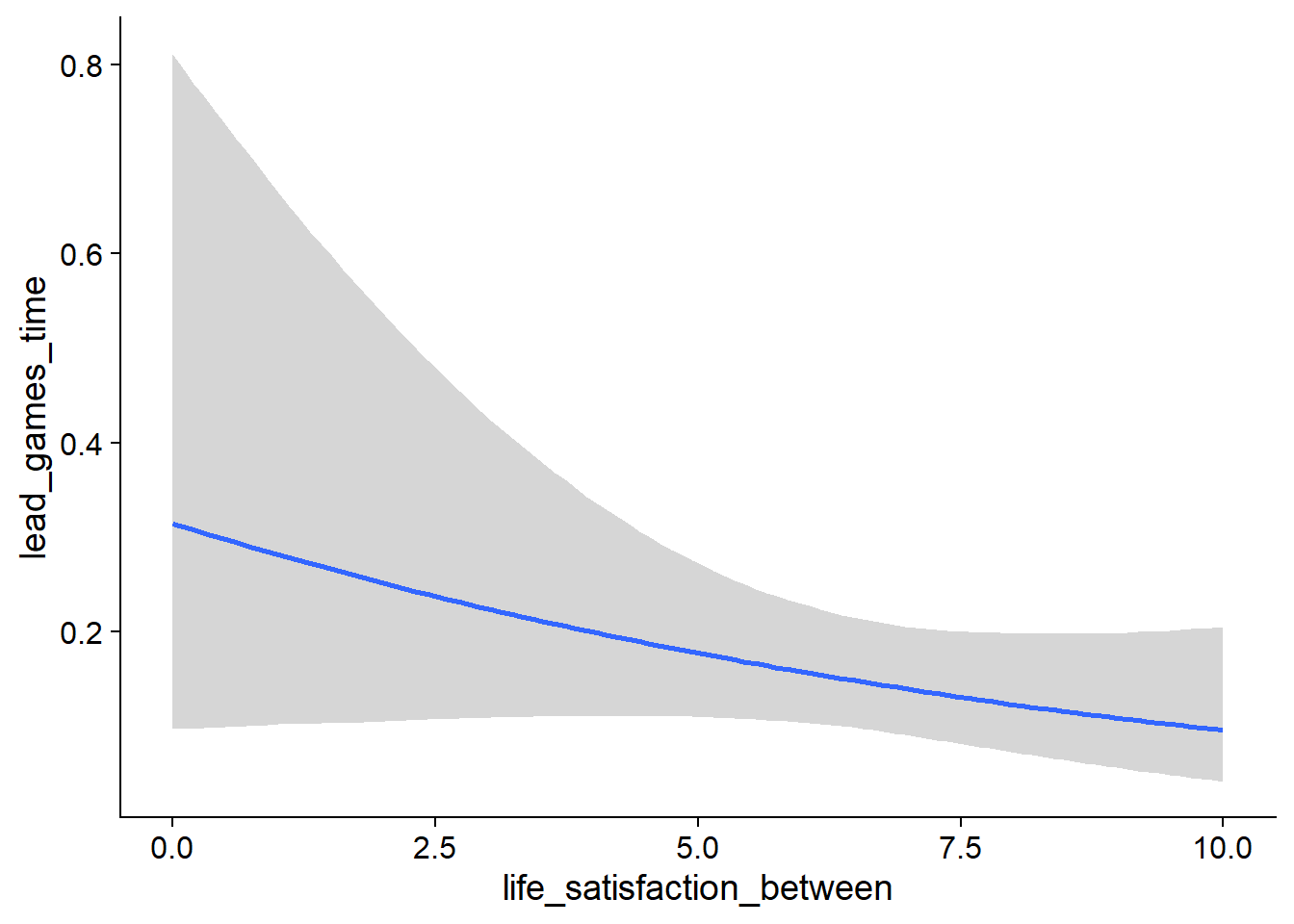
Figure 4.111: Conditional effects for Life Satisfaction-Games model
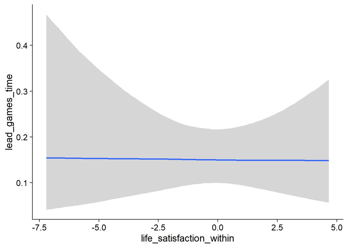
Figure 4.112: Conditional effects for Life Satisfaction-Games model
##            used  (Mb) gc trigger   (Mb)  max used   (Mb)
## Ncells  3693067 197.3    6044351  322.9   6044351  322.9
## Vcells 23779795 181.5  196534017 1499.5 255811179 1951.7
4.6 (E-)books
4.6.1 Affect
4.6.1.1 Books on affect
I had to increase the number of iterations.
books_affect <-
  brm(
    data = working_file,
    family = gaussian,
    affect ~
      1 +
      books_used_between +
      books_used_within +
      books_time_between +
      books_time_within +
      (1 +
         books_time_within +
         books_used_within
       | id),
    iter = 7000,
    warmup = 3000,
    chains = 4,
    cores = 4,
    seed = 42,
    control = list(adapt_delta = 0.95),
    file = here("models", "books_affect")
  )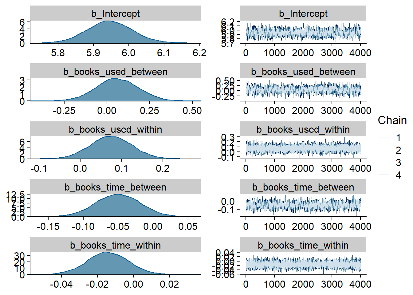
Figure 4.113: Traceplots and posterior distributions for Books-Affect model
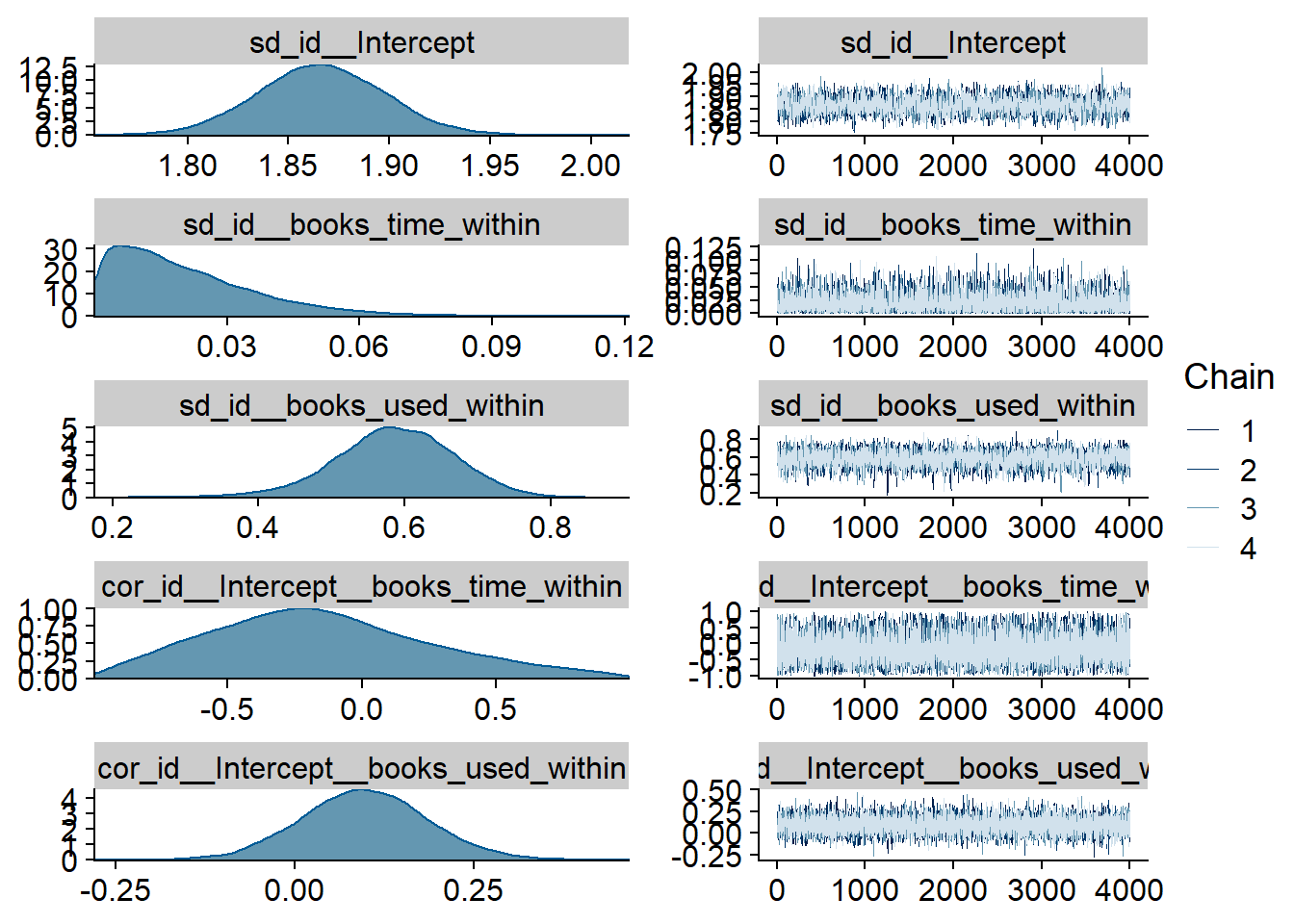
Figure 4.114: Traceplots and posterior distributions for Books-Affect model
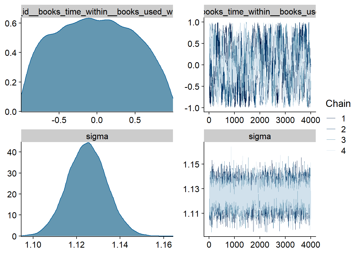
Figure 4.115: Traceplots and posterior distributions for Books-Affect model
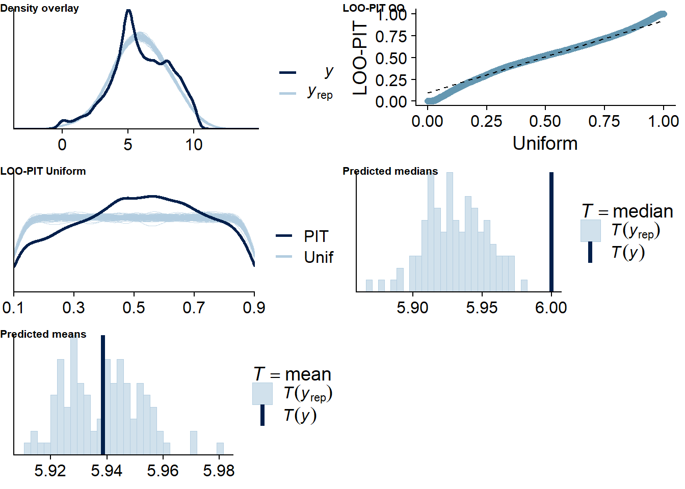
Figure 4.116: Posterior predictive checks for Books-Affect model
The outliers are in about the same range as in previous models, and the model diagnostics look good.
books_affect_loo <- loo(books_affect)
books_affect_loo
##
## Computed from 16000 by 10985 log-likelihood matrix
##
## Estimate SE
## elpd_loo -18100.9 105.7
## p_loo 2039.9 35.6
## looic 36201.8 211.4
## ------
## Monte Carlo SE of elpd_loo is NA.
##
## Pareto k diagnostic values:
## Count Pct. Min. n_eff
## (-Inf, 0.5] (good) 10554 96.1% 614
## (0.5, 0.7] (ok) 399 3.6% 166
## (0.7, 1] (bad) 30 0.3% 33
## (1, Inf) (very bad) 2 0.0% 9
## See help('pareto-k-diagnostic') for details.Below the summary.
summary(books_affect)## Family: gaussian
## Links: mu = identity; sigma = identity
## Formula: affect ~ 1 + books_used_between + books_used_within + books_time_between + books_time_within + (1 + books_time_within + books_used_within | id)
## Data: working_file (Number of observations: 10985)
## Samples: 4 chains, each with iter = 7000; warmup = 3000; thin = 1;
## total post-warmup samples = 16000
##
## Group-Level Effects:
## ~id (Number of levels: 2159)
## Estimate Est.Error l-95% CI u-95% CI Rhat Bulk_ESS Tail_ESS
## sd(Intercept) 1.87 0.03 1.81 1.93 1.00 2277 3775
## sd(books_time_within) 0.02 0.02 0.00 0.06 1.00 5067 7200
## sd(books_used_within) 0.59 0.08 0.41 0.74 1.00 3603 5386
## cor(Intercept,books_time_within) -0.15 0.41 -0.86 0.75 1.00 19382 9497
## cor(Intercept,books_used_within) 0.10 0.09 -0.07 0.27 1.00 16745 11190
## cor(books_time_within,books_used_within) -0.03 0.51 -0.89 0.87 1.02 243 1099
##
## Population-Level Effects:
## Estimate Est.Error l-95% CI u-95% CI Rhat Bulk_ESS Tail_ESS
## Intercept 5.95 0.06 5.82 6.08 1.00 1500 2698
## books_used_between 0.06 0.12 -0.18 0.30 1.00 1271 2280
## books_used_within 0.07 0.05 -0.02 0.17 1.00 19776 12900
## books_time_between -0.05 0.03 -0.11 0.01 1.00 1608 3147
## books_time_within -0.01 0.01 -0.04 0.01 1.00 23090 12615
##
## Family Specific Parameters:
## Estimate Est.Error l-95% CI u-95% CI Rhat Bulk_ESS Tail_ESS
## sigma 1.12 0.01 1.11 1.14 1.00 12209 12010
##
## Samples were drawn using sampling(NUTS). For each parameter, Bulk_ESS
## and Tail_ESS are effective sample size measures, and Rhat is the potential
## scale reduction factor on split chains (at convergence, Rhat = 1).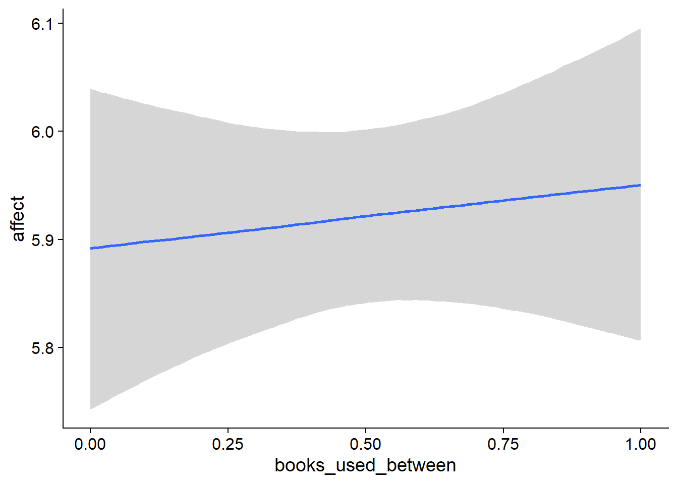
Figure 4.117: Conditional effects for Books-Affect model
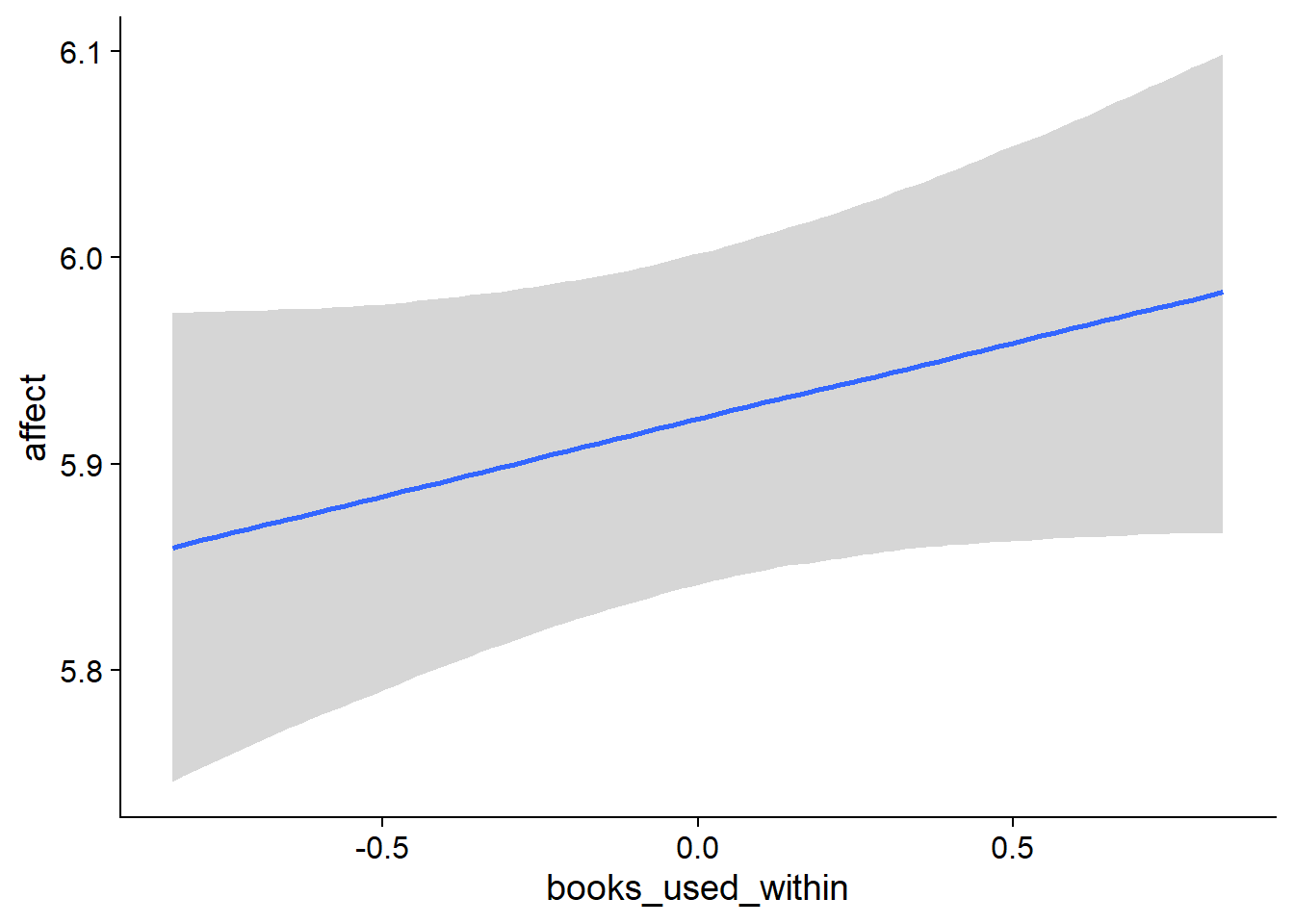
Figure 4.118: Conditional effects for Books-Affect model
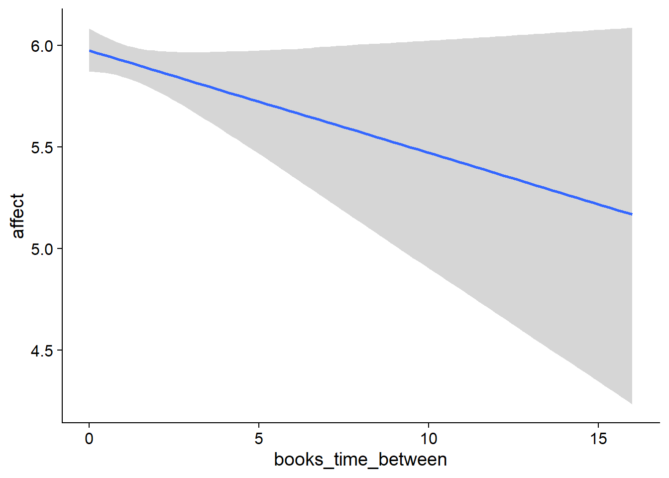
Figure 4.119: Conditional effects for Books-Affect model
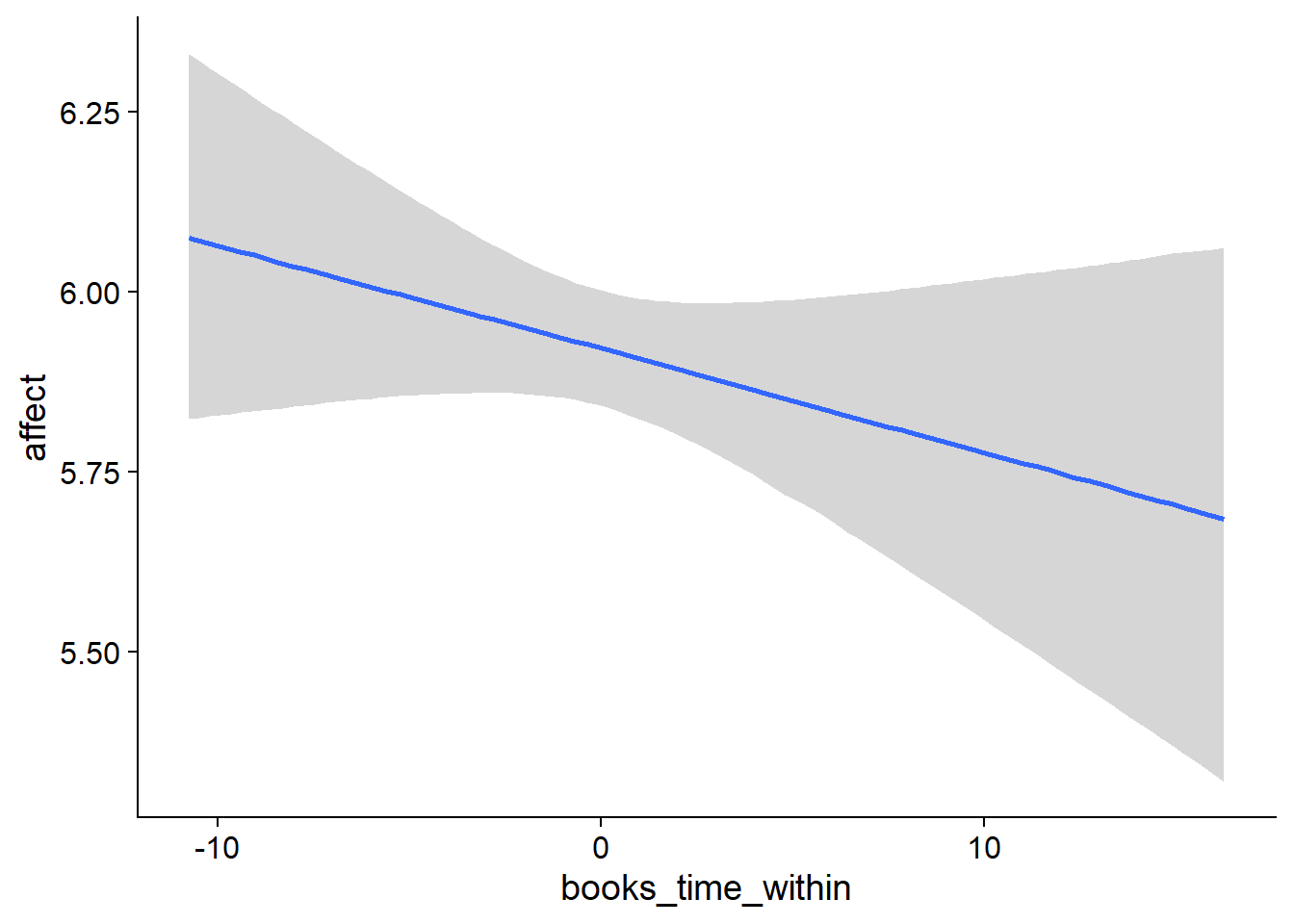
Figure 4.120: Conditional effects for Books-Affect model
##            used  (Mb) gc trigger   (Mb)  max used   (Mb)
## Ncells  3693227 197.3    6044351  322.9   6044351  322.9
## Vcells 23780884 181.5  190351213 1452.3 255811179 1951.7
4.6.1.2 Affect on books
affect_books <-
  brm(
    bf(
      # predicting continuous part
      lead_books_time ~
        1 +
        affect_between +
        affect_within +
        (1 +
           affect_within
         | id),

      # predicting hurdle part
      hu ~
        1 +
        affect_between +
        affect_within +
        (1 +
           affect_within
         | id)
    ),
    data = working_file,
    family = hurdle_gamma(),
    ,
    iter = 5000,
    warmup = 2000,
    chains = 4,
    cores = 4,
    seed = 42,
    control = list(adapt_delta = 0.95),
    file = here("models", "affect_books")
  )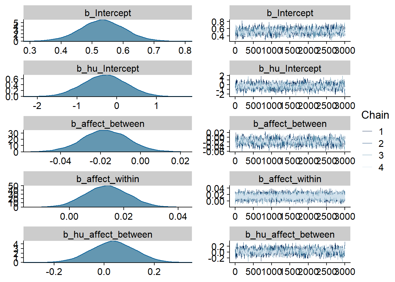
Figure 4.121: Traceplots and posterior distributions for Affect-Books model
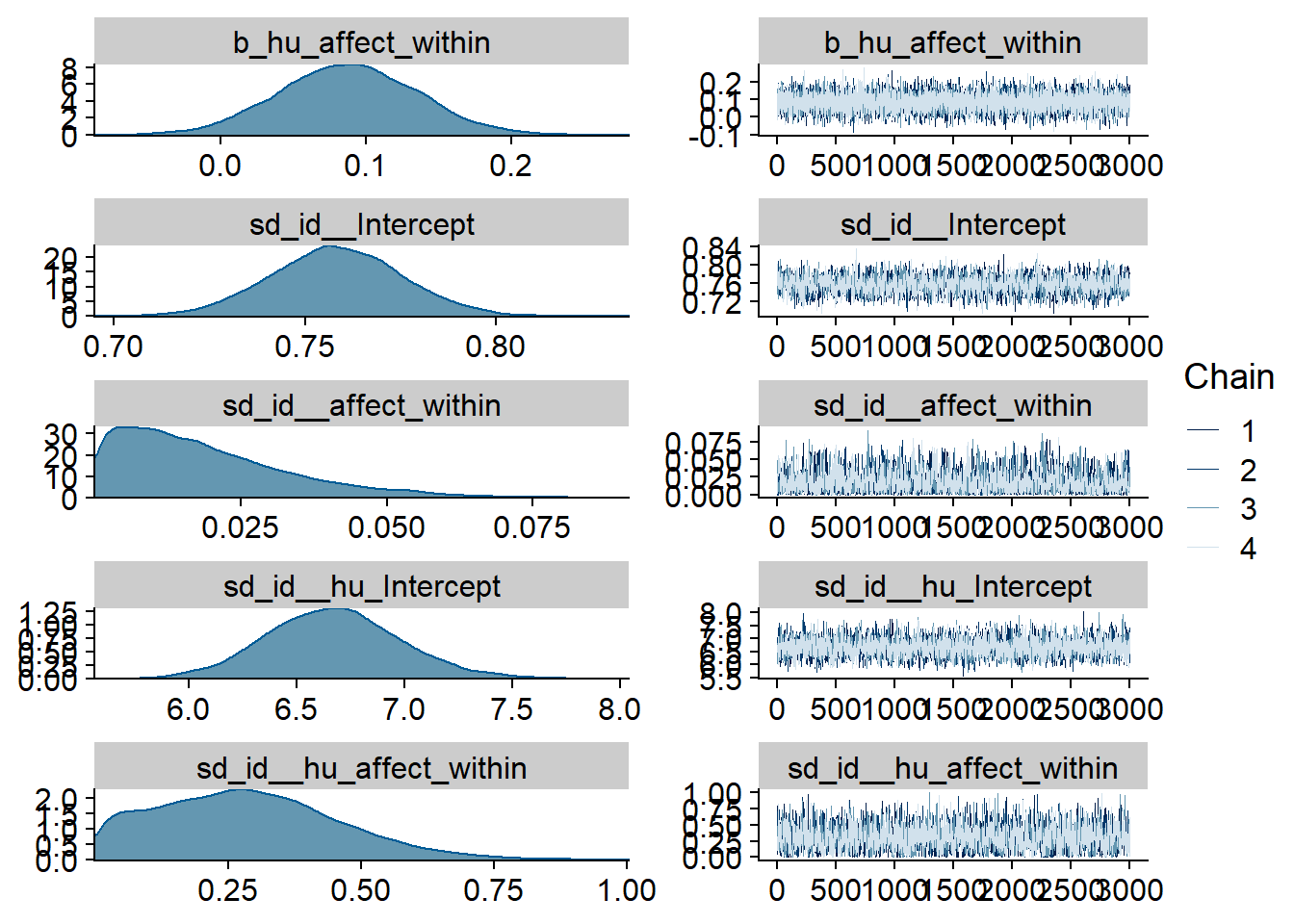
Figure 4.122: Traceplots and posterior distributions for Affect-Books model
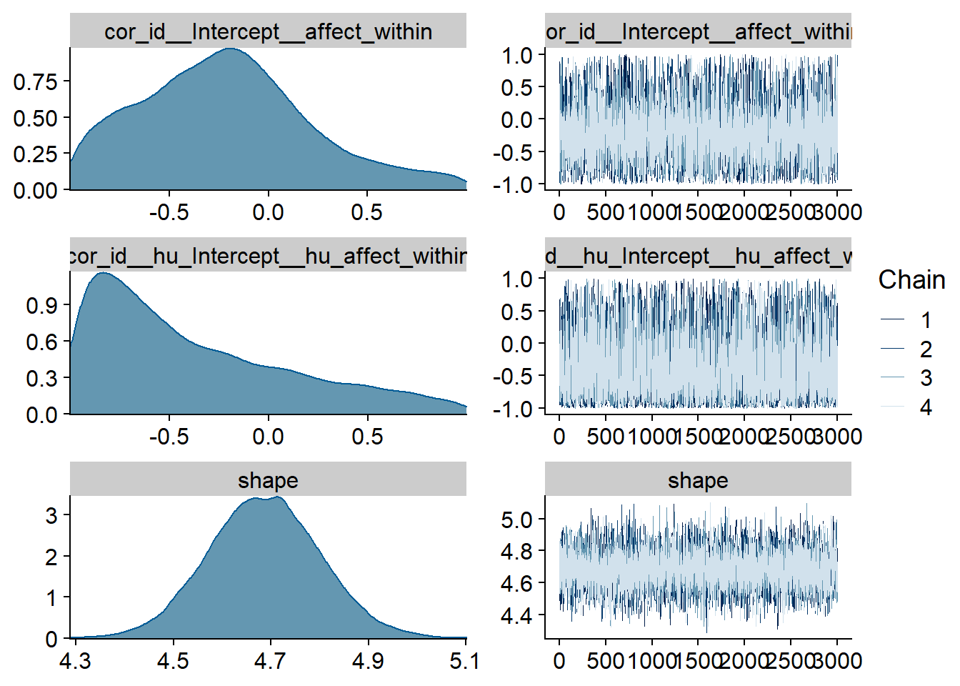
Figure 4.123: Traceplots and posterior distributions for Affect-Books model
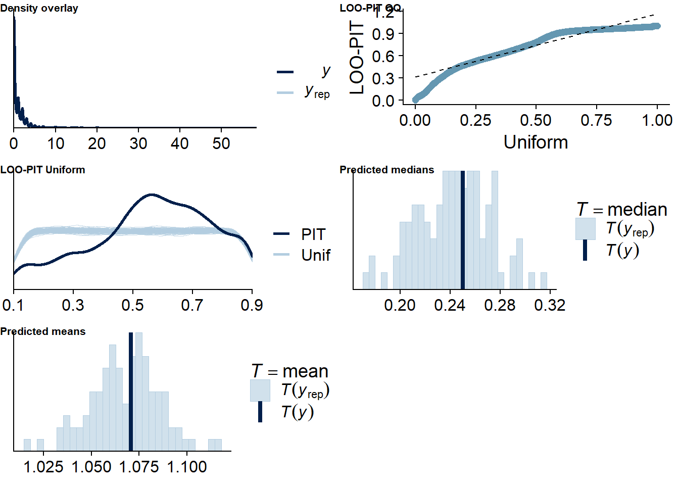
Figure 4.124: Posterior predictive checks for Affect-Books model
There are a similar number of potentially influential values as in the two previous affect models.
affect_books_loo <- loo(affect_books)
affect_books_loo
##
## Computed from 12000 by 8698 log-likelihood matrix
##
## Estimate SE
## elpd_loo -7635.6 125.7
## p_loo 2024.0 55.1
## looic 15271.3 251.3
## ------
## Monte Carlo SE of elpd_loo is NA.
##
## Pareto k diagnostic values:
## Count Pct. Min. n_eff
## (-Inf, 0.5] (good) 7598 87.4% 1032
## (0.5, 0.7] (ok) 628 7.2% 170
## (0.7, 1] (bad) 382 4.4% 11
## (1, Inf) (very bad) 90 1.0% 1
## See help('pareto-k-diagnostic') for details.Below the summary.
summary(affect_books)## Family: hurdle_gamma
## Links: mu = log; shape = identity; hu = logit
## Formula: lead_books_time ~ 1 + affect_between + affect_within + (1 + affect_within | id)
## hu ~ 1 + affect_between + affect_within + (1 + affect_within | id)
## Data: working_file (Number of observations: 8698)
## Samples: 4 chains, each with iter = 5000; warmup = 2000; thin = 1;
## total post-warmup samples = 12000
##
## Group-Level Effects:
## ~id (Number of levels: 2157)
## Estimate Est.Error l-95% CI u-95% CI Rhat Bulk_ESS Tail_ESS
## sd(Intercept) 0.76 0.02 0.72 0.79 1.00 2051 4200
## sd(affect_within) 0.02 0.01 0.00 0.05 1.00 1658 2435
## sd(hu_Intercept) 6.67 0.31 6.08 7.32 1.00 2871 5882
## sd(hu_affect_within) 0.29 0.17 0.02 0.66 1.00 1700 2910
## cor(Intercept,affect_within) -0.21 0.43 -0.93 0.78 1.00 8211 5811
## cor(hu_Intercept,hu_affect_within) -0.38 0.50 -0.97 0.79 1.00 5381 5196
##
## Population-Level Effects:
## Estimate Est.Error l-95% CI u-95% CI Rhat Bulk_ESS Tail_ESS
## Intercept 0.53 0.07 0.39 0.67 1.01 1239 2735
## hu_Intercept -0.30 0.55 -1.38 0.76 1.00 1309 2714
## affect_between -0.02 0.01 -0.04 0.00 1.01 1267 2670
## affect_within 0.01 0.01 -0.00 0.03 1.00 12692 9852
## hu_affect_between 0.03 0.09 -0.14 0.20 1.00 1291 2680
## hu_affect_within 0.09 0.05 -0.01 0.18 1.00 13720 8906
##
## Family Specific Parameters:
## Estimate Est.Error l-95% CI u-95% CI Rhat Bulk_ESS Tail_ESS
## shape 4.69 0.11 4.47 4.91 1.00 7153 8079
##
## Samples were drawn using sampling(NUTS). For each parameter, Bulk_ESS
## and Tail_ESS are effective sample size measures, and Rhat is the potential
## scale reduction factor on split chains (at convergence, Rhat = 1).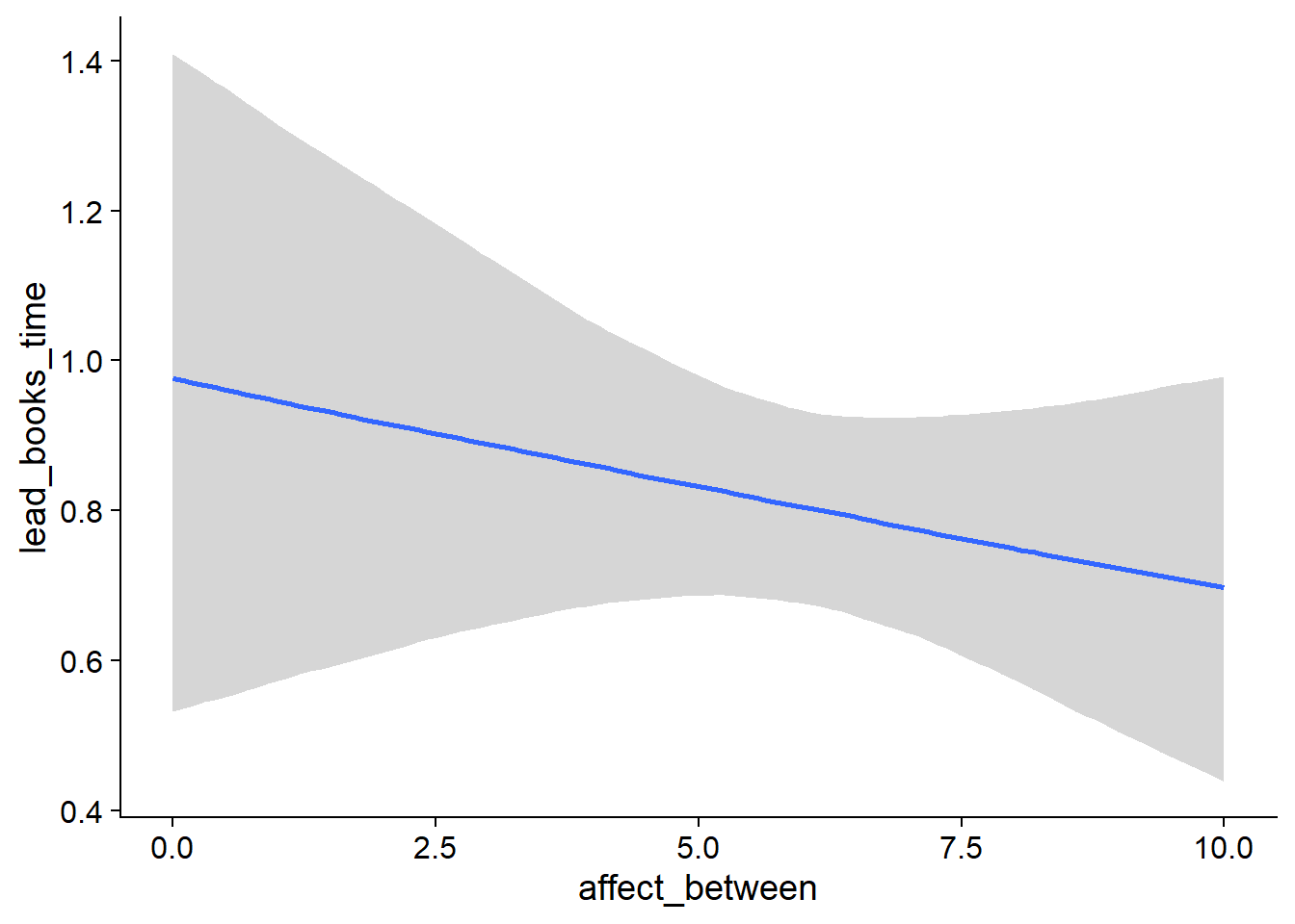
Figure 4.125: Conditional effects for Affect-Books model
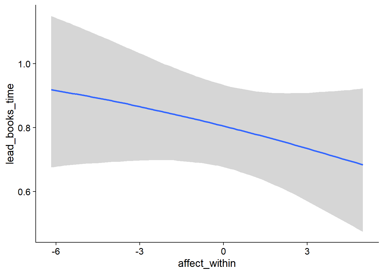
Figure 4.126: Conditional effects for Affect-Books model
##            used  (Mb) gc trigger   (Mb)  max used   (Mb)
## Ncells  3693327 197.3    6044351  322.9   6044351  322.9
## Vcells 23781809 181.5  184413447 1407.0 255811179 1951.7
4.6.2 Life satisfaction
4.6.2.1 Books on life satisfaction
books_life <-
  brm(
    data = working_file,
    family = gaussian,
    life_satisfaction ~
      1 +
      books_used_between +
      books_used_within +
      books_time_between +
      books_time_within +
      (1 +
         books_time_within +
         books_used_within
       | id),
    iter = 7000,
    warmup = 3000,
    chains = 4,
    cores = 4,
    seed = 42,
    control = list(adapt_delta = 0.95),
    file = here("models", "books_life")
  )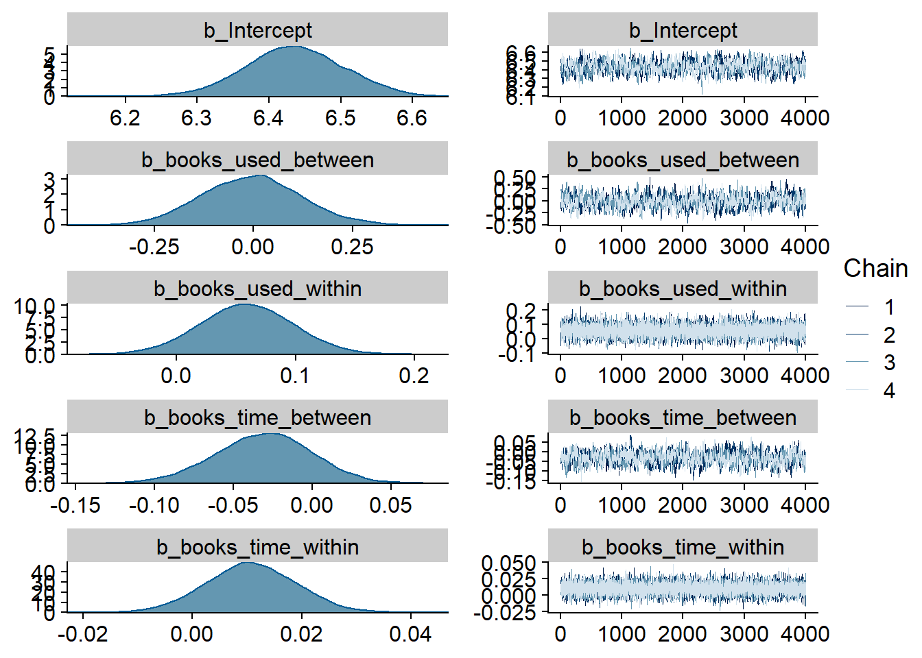
Figure 4.127: Traceplots and posterior distributions for Books-Life Satisfaction model
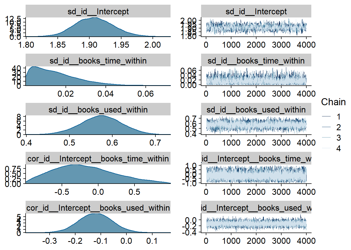
Figure 4.128: Traceplots and posterior distributions for Books-Life Satisfaction model
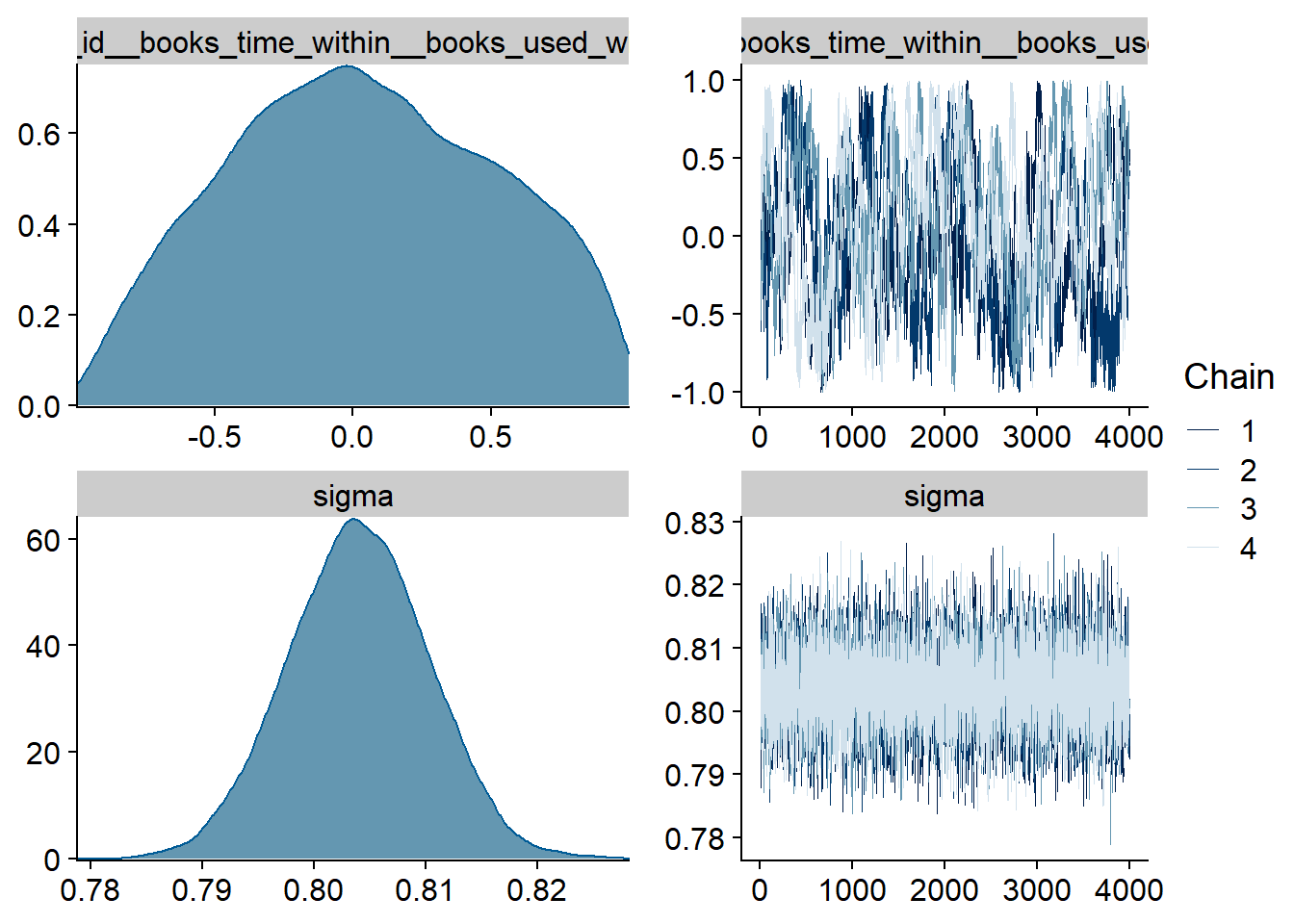
Figure 4.129: Traceplots and posterior distributions for Books-Life Satisfaction model
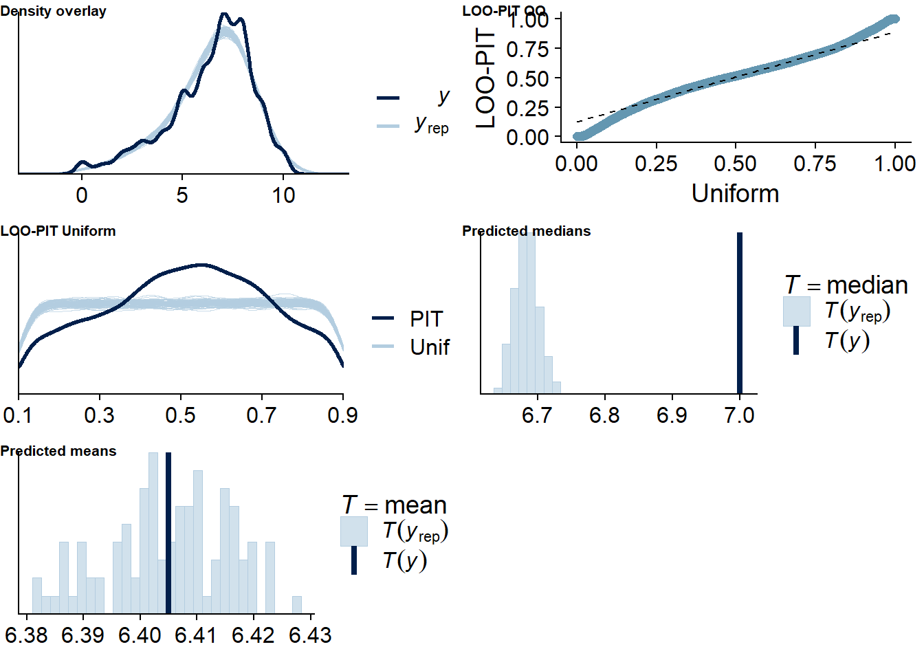
Figure 4.130: Posterior predictive checks for Books-Life Satisfaction model
The outliers are in about the same range as in previous models, and the model diagnostics look good.
books_life_loo <- loo(books_life)
books_life_loo
##
## Computed from 16000 by 10985 log-likelihood matrix
##
## Estimate SE
## elpd_loo -14543.5 145.4
## p_loo 2218.4 51.9
## looic 29087.0 290.9
## ------
## Monte Carlo SE of elpd_loo is NA.
##
## Pareto k diagnostic values:
## Count Pct. Min. n_eff
## (-Inf, 0.5] (good) 10377 94.5% 680
## (0.5, 0.7] (ok) 494 4.5% 166
## (0.7, 1] (bad) 101 0.9% 13
## (1, Inf) (very bad) 13 0.1% 2
## See help('pareto-k-diagnostic') for details.Below the summary.
summary(books_life)## Family: gaussian
## Links: mu = identity; sigma = identity
## Formula: life_satisfaction ~ 1 + books_used_between + books_used_within + books_time_between + books_time_within + (1 + books_time_within + books_used_within | id)
## Data: working_file (Number of observations: 10985)
## Samples: 4 chains, each with iter = 7000; warmup = 3000; thin = 1;
## total post-warmup samples = 16000
##
## Group-Level Effects:
## ~id (Number of levels: 2159)
## Estimate Est.Error l-95% CI u-95% CI Rhat Bulk_ESS Tail_ESS
## sd(Intercept) 1.91 0.03 1.85 1.97 1.00 1083 2354
## sd(books_time_within) 0.01 0.01 0.00 0.04 1.00 3790 6864
## sd(books_used_within) 0.57 0.05 0.48 0.67 1.00 2990 7917
## cor(Intercept,books_time_within) -0.19 0.42 -0.88 0.72 1.00 13557 9347
## cor(Intercept,books_used_within) -0.12 0.07 -0.25 0.01 1.00 13423 11938
## cor(books_time_within,books_used_within) 0.04 0.47 -0.82 0.89 1.04 118 358
##
## Population-Level Effects:
## Estimate Est.Error l-95% CI u-95% CI Rhat Bulk_ESS Tail_ESS
## Intercept 6.44 0.07 6.31 6.57 1.01 560 1236
## books_used_between -0.01 0.12 -0.24 0.25 1.01 612 1396
## books_used_within 0.06 0.04 -0.02 0.14 1.00 13260 11309
## books_time_between -0.03 0.03 -0.09 0.03 1.00 788 1582
## books_time_within 0.01 0.01 -0.01 0.03 1.00 18096 11991
##
## Family Specific Parameters:
## Estimate Est.Error l-95% CI u-95% CI Rhat Bulk_ESS Tail_ESS
## sigma 0.80 0.01 0.79 0.82 1.00 12610 11889
##
## Samples were drawn using sampling(NUTS). For each parameter, Bulk_ESS
## and Tail_ESS are effective sample size measures, and Rhat is the potential
## scale reduction factor on split chains (at convergence, Rhat = 1).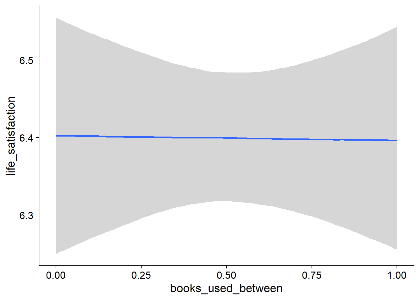
Figure 4.131: Conditional effects for Books-Life Satisfaction model
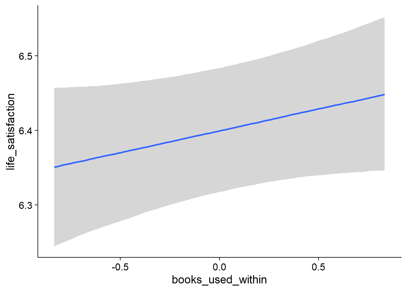
Figure 4.132: Conditional effects for Books-Life Satisfaction model
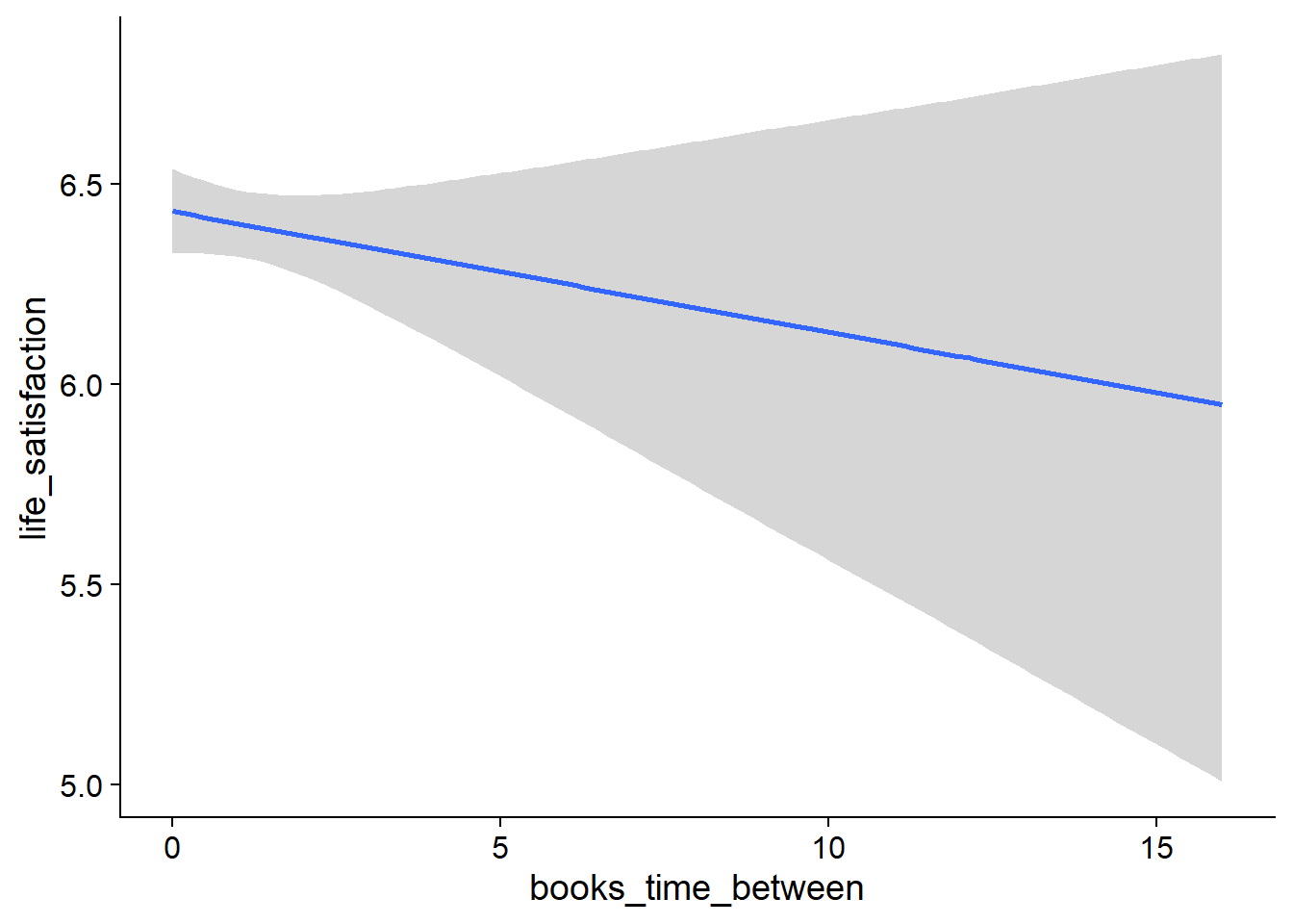
Figure 4.133: Conditional effects for Books-Life Satisfaction model
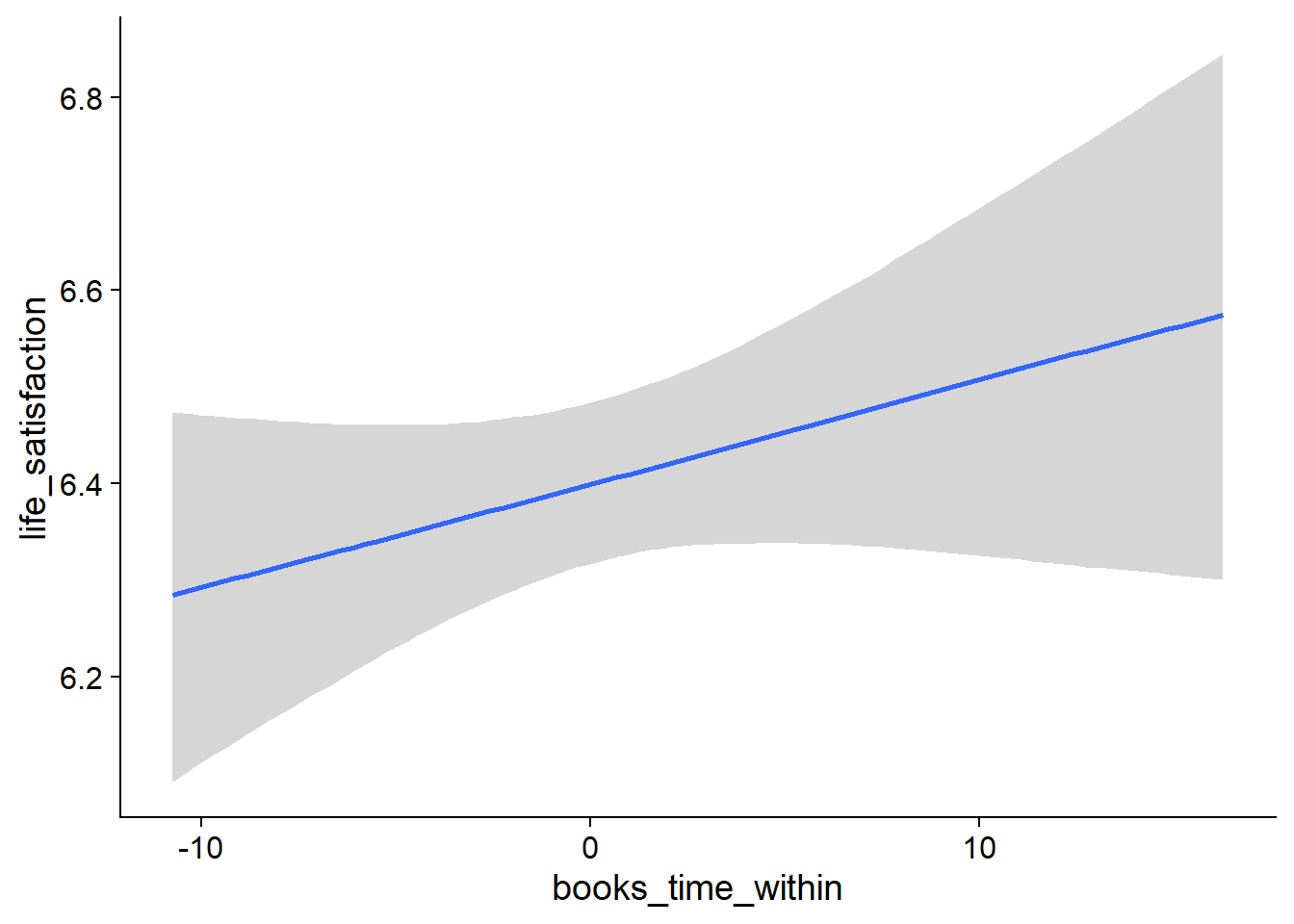
Figure 4.134: Conditional effects for Books-Life Satisfaction model
##            used  (Mb) gc trigger   (Mb)  max used   (Mb)
## Ncells  3693400 197.3    6044351  322.9   6044351  322.9
## Vcells 23782743 181.5  178714130 1363.5 255811179 1951.7
4.6.2.2 Life satisfaction on books
life_books <-
  brm(
    bf(
      # predicting continuous part
      lead_books_time ~
        1 +
        life_satisfaction_between +
        life_satisfaction_within +
        (1 +
           life_satisfaction_within
         | id),

      # predicting hurdle part
      hu ~
        1 +
        life_satisfaction_between +
        life_satisfaction_within +
        (1 +
           life_satisfaction_within
         | id)
    ),
    data = working_file,
    family = hurdle_gamma(),
    ,
    iter = 5000,
    warmup = 2000,
    chains = 4,
    cores = 4,
    seed = 42,
    control = list(adapt_delta = 0.95),
    file = here("models", "life_books")
  )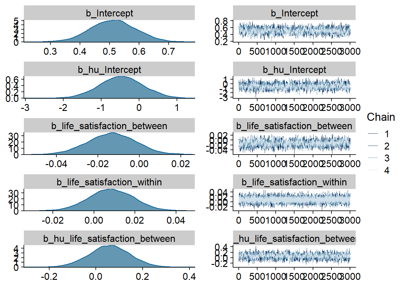
Figure 4.135: Traceplots and posterior distributions for Life Satisfaction-Books model
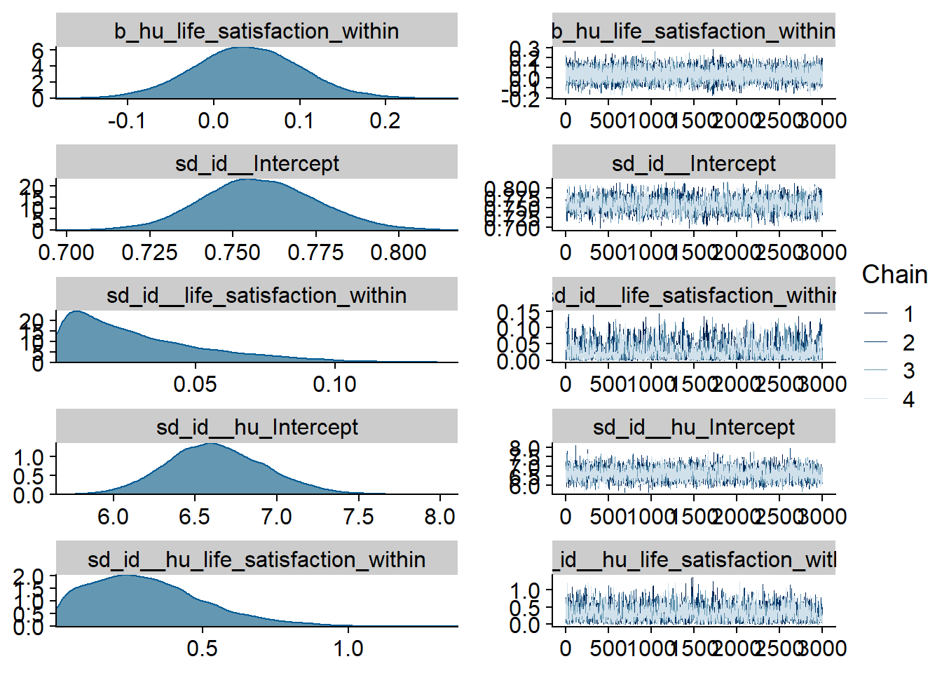
Figure 4.136: Traceplots and posterior distributions for Life Satisfaction-Books model
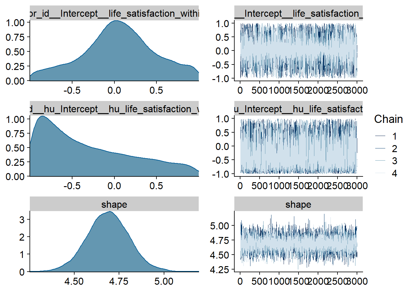
Figure 4.137: Traceplots and posterior distributions for Life Satisfaction-Books model
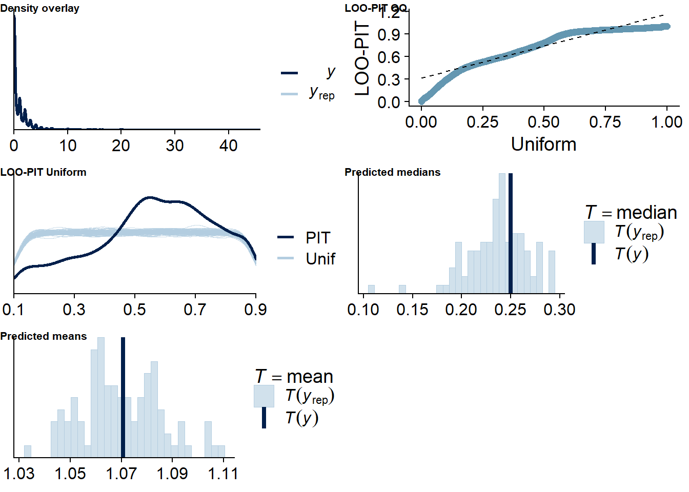
Figure 4.138: Posterior predictive checks for Life Satisfaction-Books model
The outliers are in about the same range as in the more recent models.
life_books_loo <- loo(life_books)
life_books_loo
##
## Computed from 12000 by 8698 log-likelihood matrix
##
## Estimate SE
## elpd_loo -7632.0 124.9
## p_loo 2011.8 54.0
## looic 15264.1 249.8
## ------
## Monte Carlo SE of elpd_loo is NA.
##
## Pareto k diagnostic values:
## Count Pct. Min. n_eff
## (-Inf, 0.5] (good) 7601 87.4% 403
## (0.5, 0.7] (ok) 627 7.2% 200
## (0.7, 1] (bad) 380 4.4% 14
## (1, Inf) (very bad) 90 1.0% 2
## See help('pareto-k-diagnostic') for details.Below the summary.
summary(life_books)## Family: hurdle_gamma
## Links: mu = log; shape = identity; hu = logit
## Formula: lead_books_time ~ 1 + life_satisfaction_between + life_satisfaction_within + (1 + life_satisfaction_within | id)
## hu ~ 1 + life_satisfaction_between + life_satisfaction_within + (1 + life_satisfaction_within | id)
## Data: working_file (Number of observations: 8698)
## Samples: 4 chains, each with iter = 5000; warmup = 2000; thin = 1;
## total post-warmup samples = 12000
##
## Group-Level Effects:
## ~id (Number of levels: 2157)
## Estimate Est.Error l-95% CI u-95% CI Rhat Bulk_ESS Tail_ESS
## sd(Intercept) 0.76 0.02 0.73 0.79 1.00 2216 3704
## sd(life_satisfaction_within) 0.03 0.02 0.00 0.09 1.00 1203 1793
## sd(hu_Intercept) 6.63 0.30 6.07 7.25 1.00 3357 6186
## sd(hu_life_satisfaction_within) 0.31 0.20 0.02 0.77 1.00 2177 4112
## cor(Intercept,life_satisfaction_within) 0.05 0.44 -0.85 0.91 1.00 9588 5808
## cor(hu_Intercept,hu_life_satisfaction_within) -0.31 0.54 -0.98 0.86 1.00 6643 7206
##
## Population-Level Effects:
## Estimate Est.Error l-95% CI u-95% CI Rhat Bulk_ESS Tail_ESS
## Intercept 0.51 0.08 0.36 0.66 1.00 1112 2553
## hu_Intercept -0.47 0.58 -1.60 0.65 1.00 1341 2913
## life_satisfaction_between -0.01 0.01 -0.04 0.01 1.01 1148 2610
## life_satisfaction_within 0.01 0.01 -0.01 0.03 1.00 14238 9376
## hu_life_satisfaction_between 0.06 0.09 -0.12 0.23 1.01 1292 2599
## hu_life_satisfaction_within 0.04 0.06 -0.08 0.16 1.00 14476 9065
##
## Family Specific Parameters:
## Estimate Est.Error l-95% CI u-95% CI Rhat Bulk_ESS Tail_ESS
## shape 4.69 0.12 4.46 4.92 1.00 6637 7916
##
## Samples were drawn using sampling(NUTS). For each parameter, Bulk_ESS
## and Tail_ESS are effective sample size measures, and Rhat is the potential
## scale reduction factor on split chains (at convergence, Rhat = 1).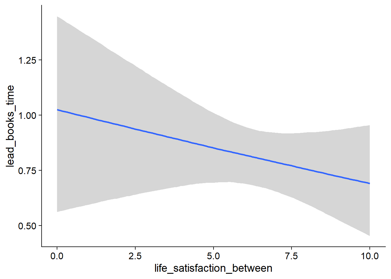
Figure 4.139: Conditional effects for Life Satisfaction-Books model
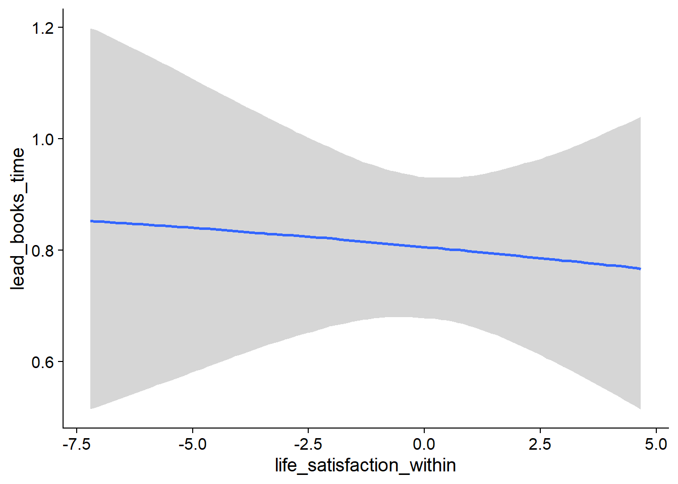
Figure 4.140: Conditional effects for Life Satisfaction-Books model
##            used  (Mb) gc trigger   (Mb)  max used   (Mb)
## Ncells  3693500 197.3    6044351  322.9   6044351  322.9
## Vcells 23783723 181.5  173243028 1321.8 255811179 1951.7
4.7 Magazines
4.7.1 Affect
4.7.1.1 Magazines on affect
I had to increase the number of iterations again.
magazines_affect <-
  brm(
    data = working_file,
    family = gaussian,
    affect ~
      1 +
      magazines_used_between +
      magazines_used_within +
      magazines_time_between +
      magazines_time_within +
      (1 +
         magazines_time_within +
         magazines_used_within
       | id),
    iter = 7000,
    warmup = 3000,
    chains = 4,
    cores = 4,
    seed = 42,
    control = list(adapt_delta = 0.95),
    file = here("models", "magazines_affect")
  )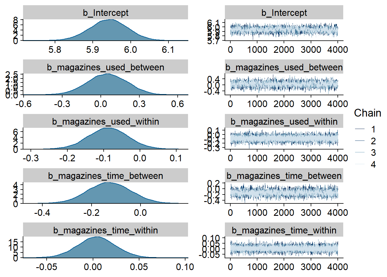
Figure 4.141: Traceplots and posterior distributions for Magazines-Affect model
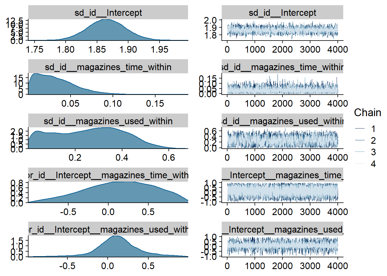
Figure 4.142: Traceplots and posterior distributions for Magazines-Affect model
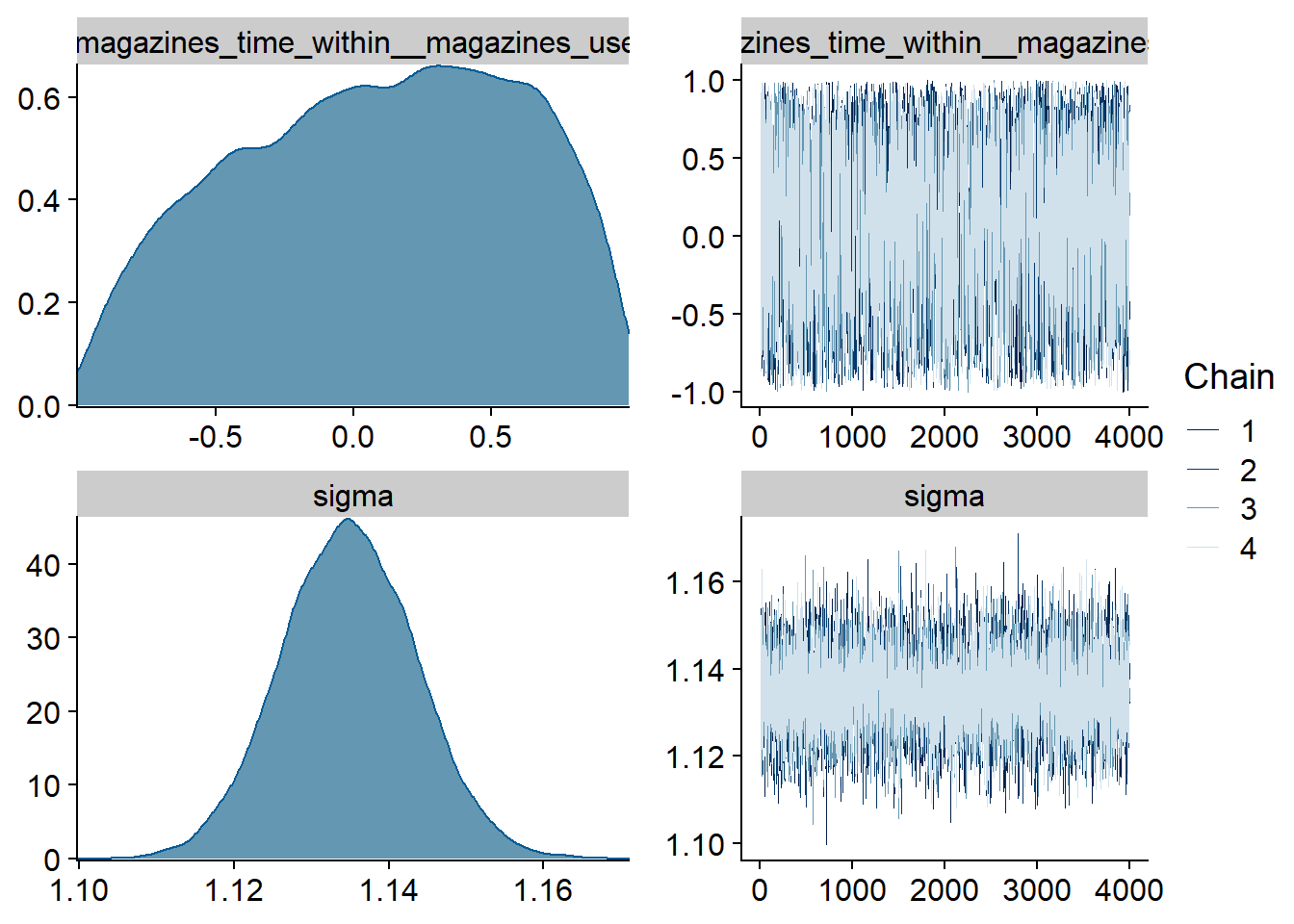
Figure 4.143: Traceplots and posterior distributions for Magazines-Affect model
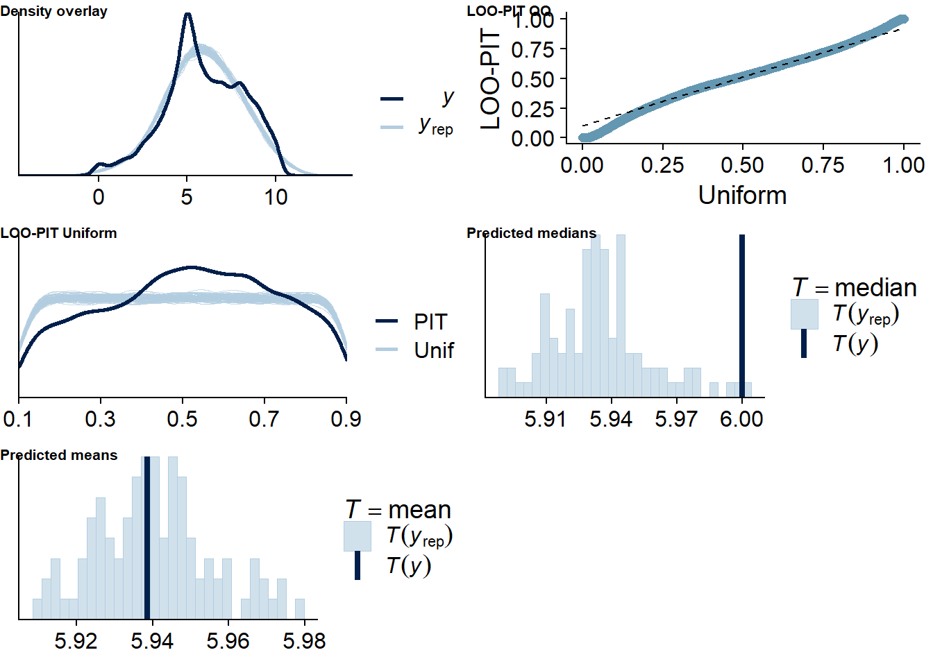
Figure 4.144: Posterior predictive checks for Magazines-Affect model
The outliers are in about the same range as in previous models, and the model diagnostics look good.
magazines_affect_loo <- loo(magazines_affect)
magazines_affect_loo
##
## Computed from 16000 by 10985 log-likelihood matrix
##
## Estimate SE
## elpd_loo -18119.3 105.3
## p_loo 1930.1 33.8
## looic 36238.6 210.5
## ------
## Monte Carlo SE of elpd_loo is NA.
##
## Pareto k diagnostic values:
## Count Pct. Min. n_eff
## (-Inf, 0.5] (good) 10652 97.0% 593
## (0.5, 0.7] (ok) 310 2.8% 172
## (0.7, 1] (bad) 22 0.2% 42
## (1, Inf) (very bad) 1 0.0% 41
## See help('pareto-k-diagnostic') for details.Below the summary.
summary(magazines_affect)## Family: gaussian
## Links: mu = identity; sigma = identity
## Formula: affect ~ 1 + magazines_used_between + magazines_used_within + magazines_time_between + magazines_time_within + (1 + magazines_time_within + magazines_used_within | id)
## Data: working_file (Number of observations: 10985)
## Samples: 4 chains, each with iter = 7000; warmup = 3000; thin = 1;
## total post-warmup samples = 16000
##
## Group-Level Effects:
## ~id (Number of levels: 2159)
## Estimate Est.Error l-95% CI u-95% CI Rhat Bulk_ESS Tail_ESS
## sd(Intercept) 1.87 0.03 1.81 1.93 1.00 3196 5959
## sd(magazines_time_within) 0.03 0.02 0.00 0.09 1.00 6015 8989
## sd(magazines_used_within) 0.26 0.15 0.01 0.52 1.00 2038 5568
## cor(Intercept,magazines_time_within) 0.14 0.43 -0.74 0.88 1.00 25152 11231
## cor(Intercept,magazines_used_within) 0.12 0.28 -0.50 0.74 1.00 14407 6731
## cor(magazines_time_within,magazines_used_within) 0.09 0.50 -0.85 0.91 1.00 2953 6285
##
## Population-Level Effects:
## Estimate Est.Error l-95% CI u-95% CI Rhat Bulk_ESS Tail_ESS
## Intercept 5.94 0.05 5.84 6.04 1.00 2393 4596
## magazines_used_between 0.05 0.16 -0.26 0.35 1.00 2532 4981
## magazines_used_within -0.09 0.05 -0.20 0.02 1.00 30880 12774
## magazines_time_between -0.13 0.09 -0.30 0.04 1.00 2787 5640
## magazines_time_within 0.00 0.02 -0.04 0.04 1.00 26087 13136
##
## Family Specific Parameters:
## Estimate Est.Error l-95% CI u-95% CI Rhat Bulk_ESS Tail_ESS
## sigma 1.13 0.01 1.12 1.15 1.00 13152 12940
##
## Samples were drawn using sampling(NUTS). For each parameter, Bulk_ESS
## and Tail_ESS are effective sample size measures, and Rhat is the potential
## scale reduction factor on split chains (at convergence, Rhat = 1).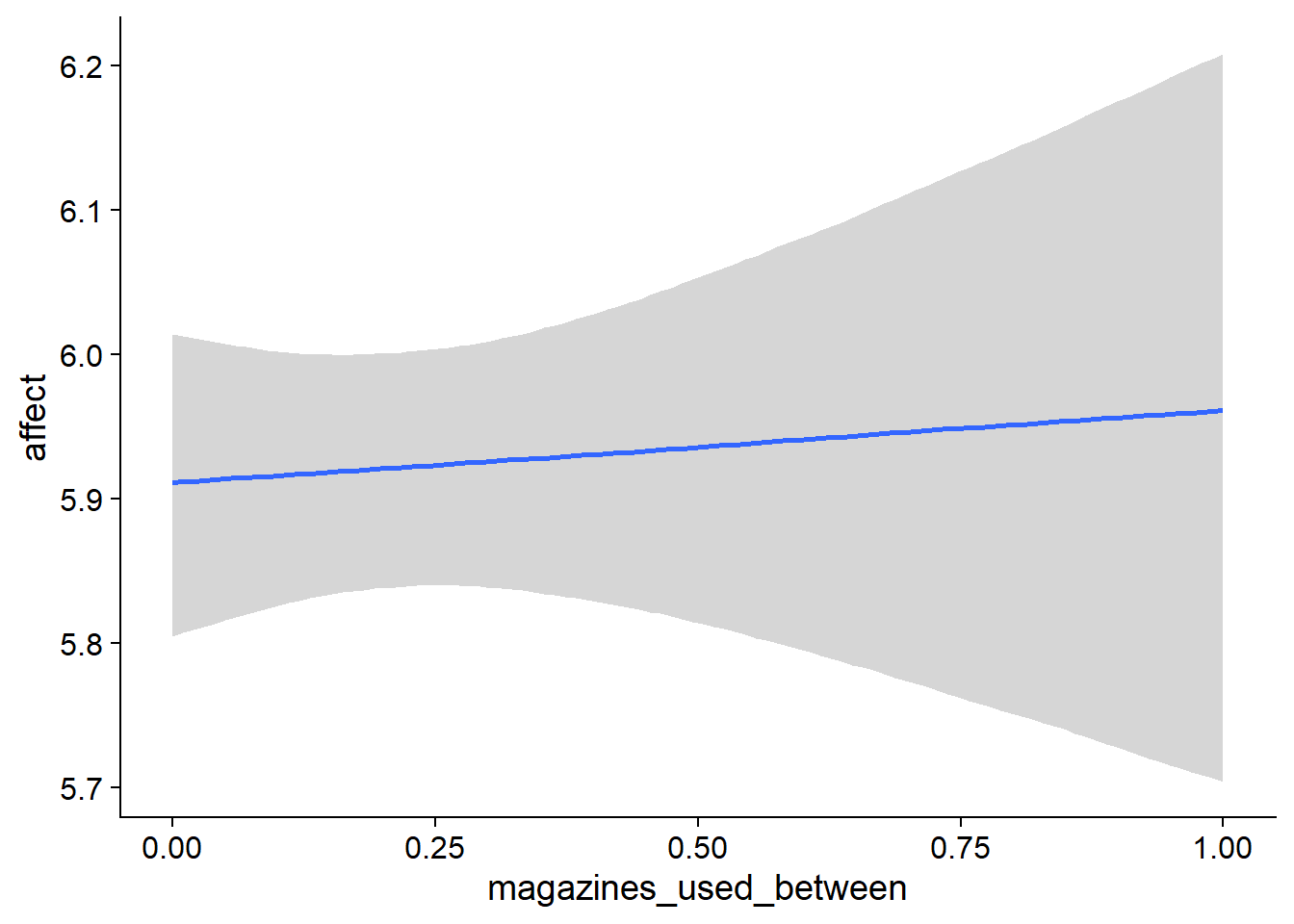
Figure 4.145: Conditional effects for Magazines-Affect model
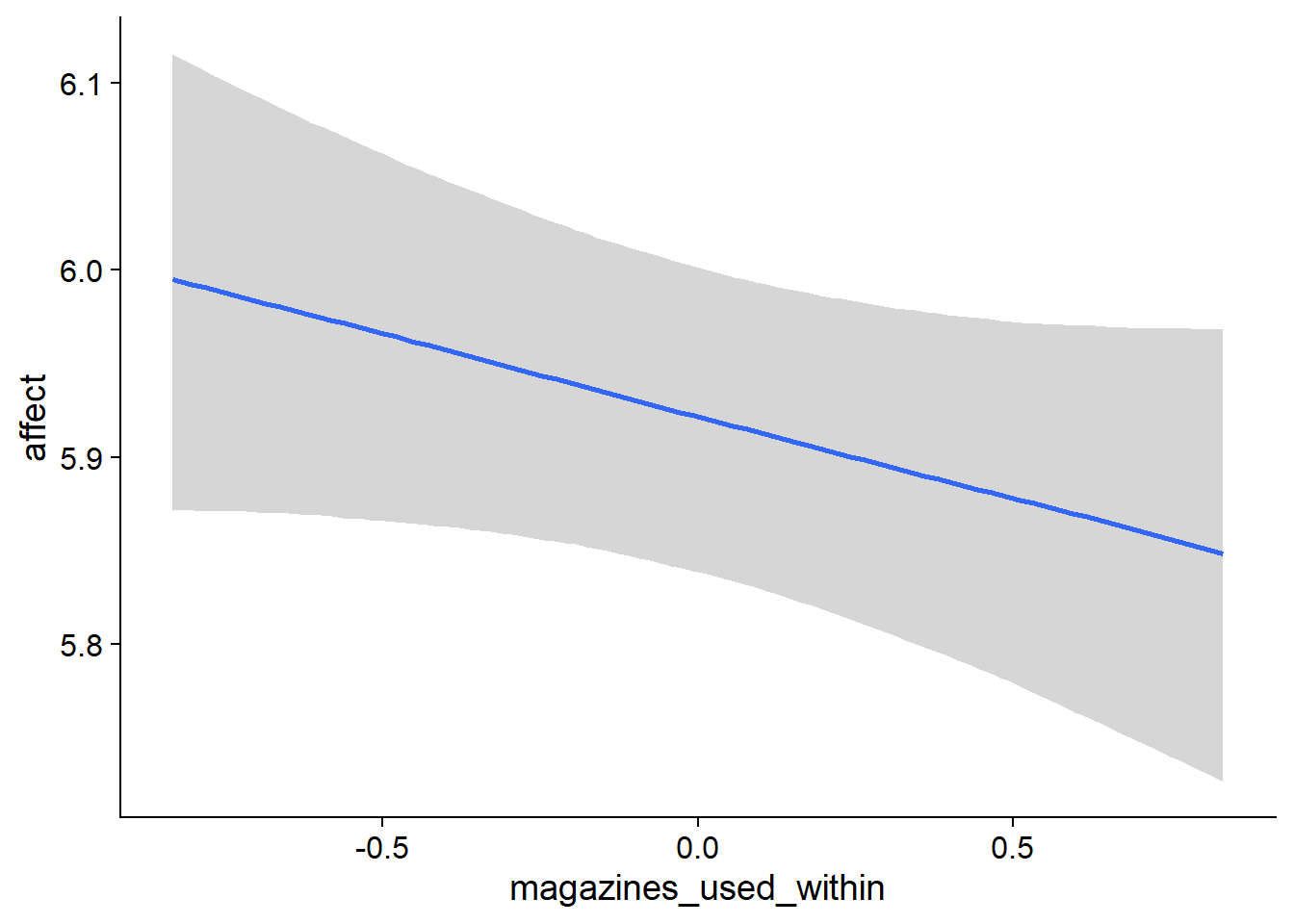
Figure 4.146: Conditional effects for Magazines-Affect model
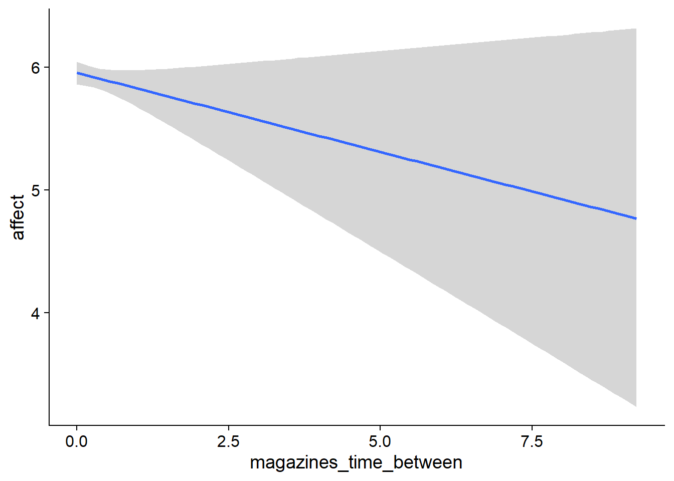
Figure 4.147: Conditional effects for Magazines-Affect model
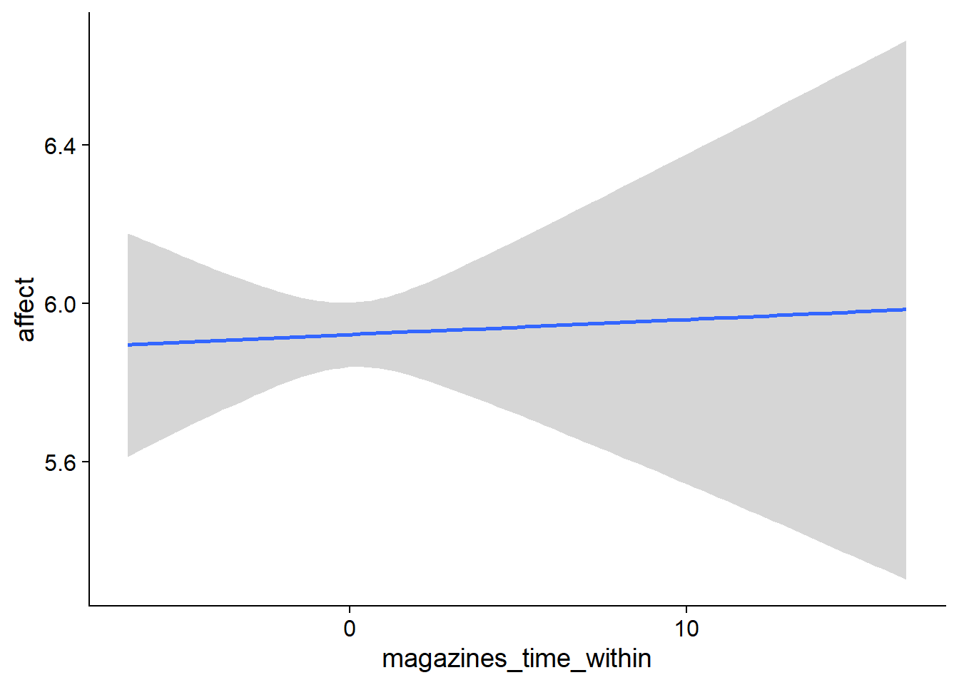
Figure 4.148: Conditional effects for Magazines-Affect model
##            used  (Mb) gc trigger   (Mb)  max used   (Mb)
## Ncells  3693624 197.3    6044351  322.9   6044351  322.9
## Vcells 23784774 181.5  201648544 1538.5 255811179 1951.7
4.7.1.2 Affect on magazines
affect_magazines <-
  brm(
    bf(
      # predicting continuous part
      lead_magazines_time ~
        1 +
        affect_between +
        affect_within +
        (1 +
           affect_within
         | id),

      # predicting hurdle part
      hu ~
        1 +
        affect_between +
        affect_within +
        (1 +
           affect_within
         | id)
    ),
    data = working_file,
    family = hurdle_gamma(),
    ,
    iter = 5000,
    warmup = 2000,
    chains = 4,
    cores = 4,
    seed = 42,
    control = list(adapt_delta = 0.95),
    file = here("models", "affect_magazines")
  )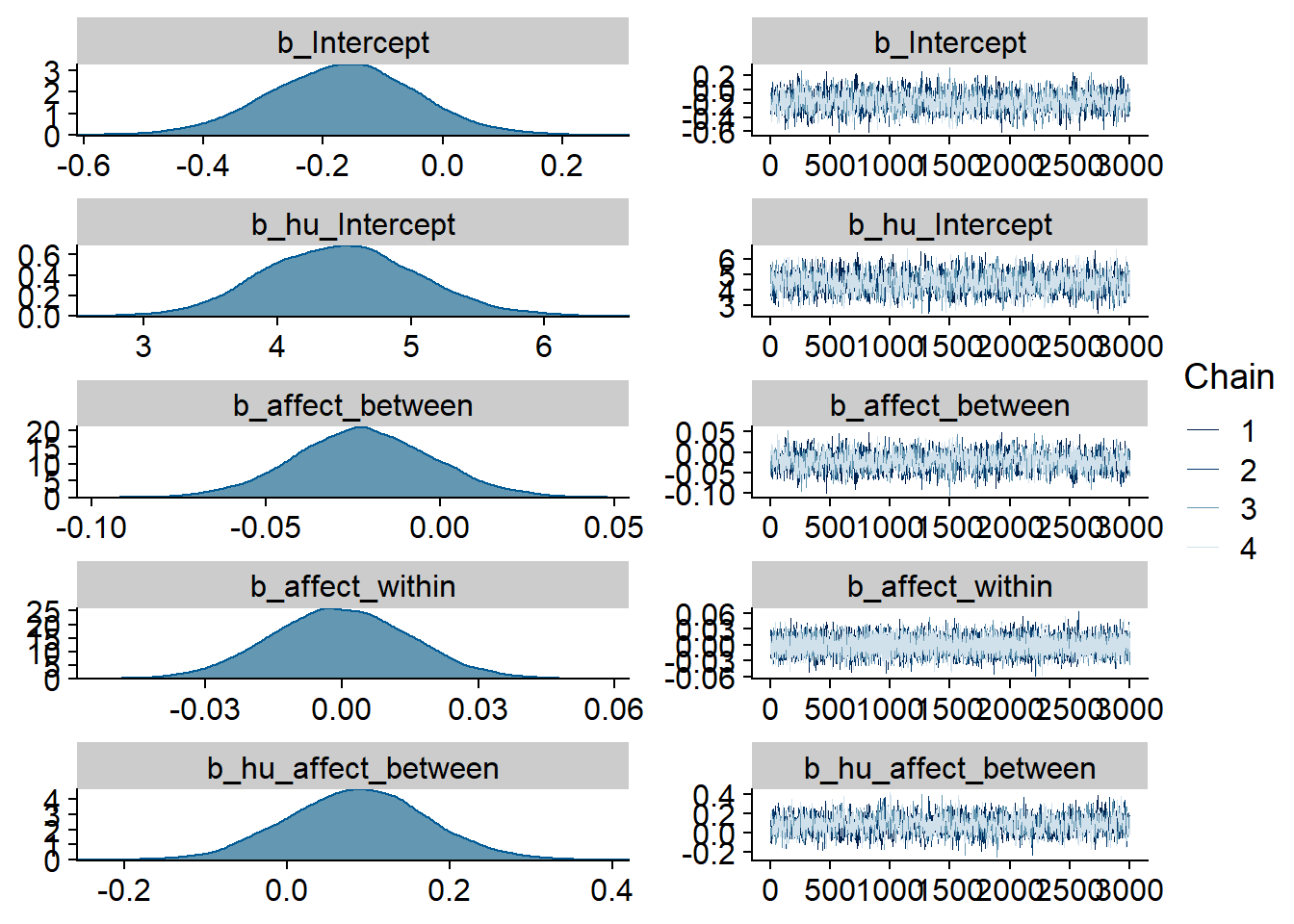
Figure 4.149: Traceplots and posterior distributions for Affect-Magazines model
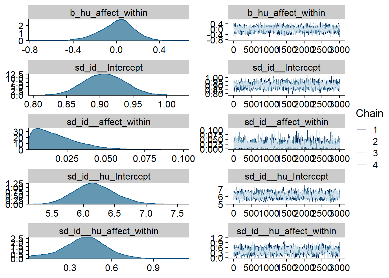
Figure 4.150: Traceplots and posterior distributions for Affect-Magazines model
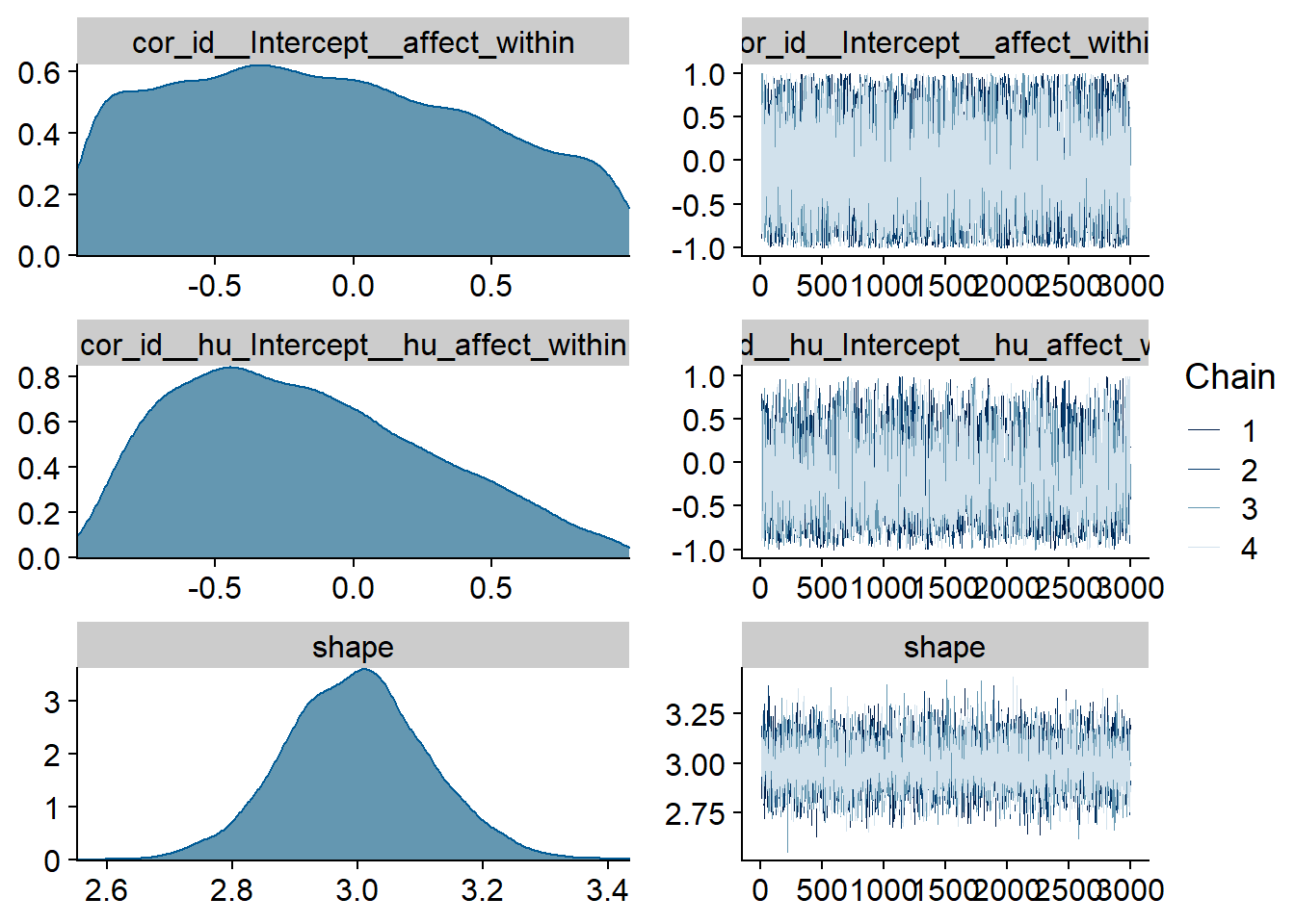
Figure 4.151: Traceplots and posterior distributions for Affect-Magazines model
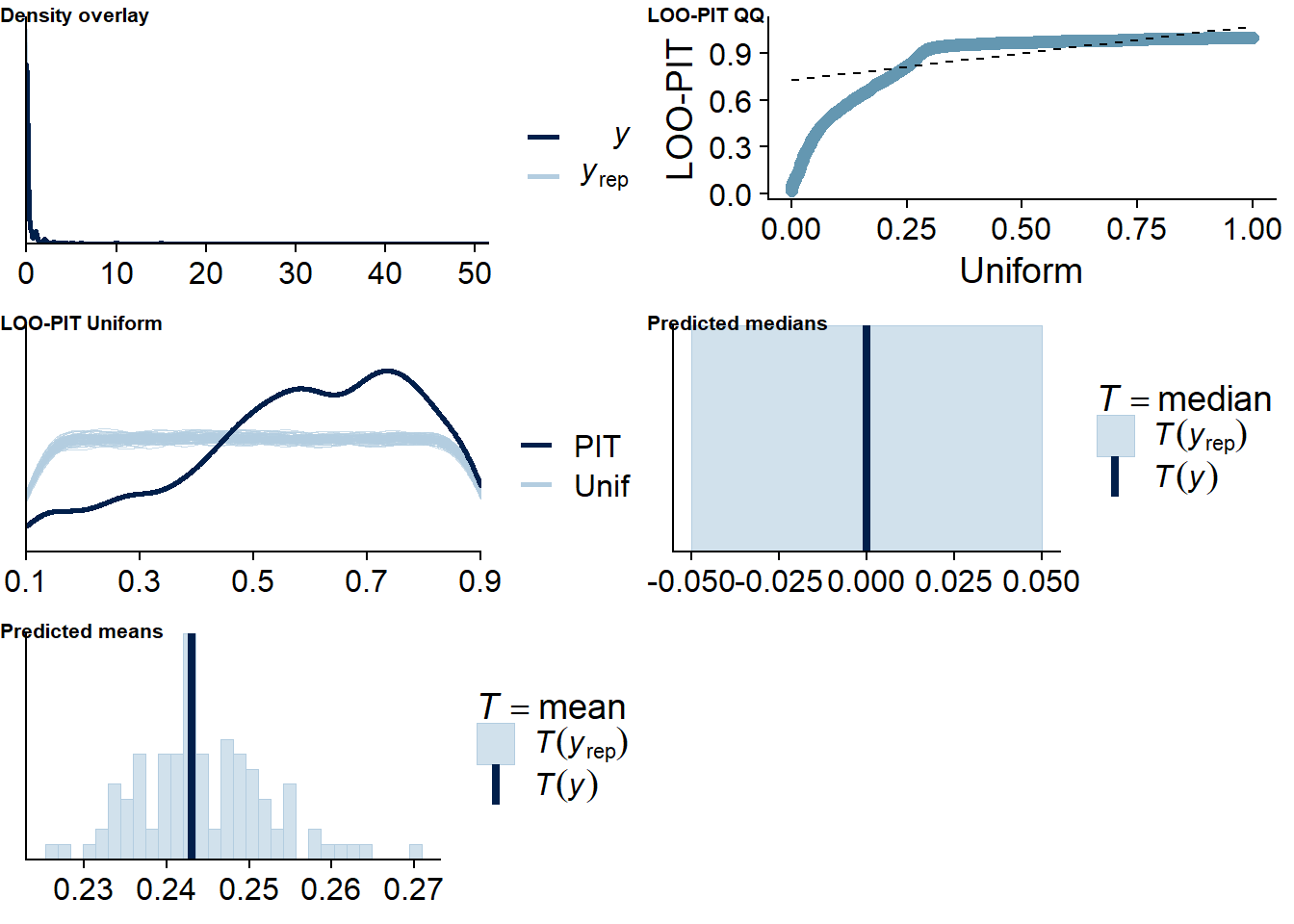
Figure 4.152: Posterior predictive checks for Affect-Magazines model
There are more potentially influential values than in earlier models, but similar to recent models.
affect_magazines_loo <- loo(affect_magazines)
affect_magazines_loo
##
## Computed from 12000 by 8698 log-likelihood matrix
##
## Estimate SE
## elpd_loo -3102.2 96.4
## p_loo 1262.8 45.9
## looic 6204.4 192.8
## ------
## Monte Carlo SE of elpd_loo is NA.
##
## Pareto k diagnostic values:
## Count Pct. Min. n_eff
## (-Inf, 0.5] (good) 7658 88.0% 1038
## (0.5, 0.7] (ok) 734 8.4% 243
## (0.7, 1] (bad) 234 2.7% 16
## (1, Inf) (very bad) 72 0.8% 1
## See help('pareto-k-diagnostic') for details.Below the summary.
summary(affect_magazines)## Family: hurdle_gamma
## Links: mu = log; shape = identity; hu = logit
## Formula: lead_magazines_time ~ 1 + affect_between + affect_within + (1 + affect_within | id)
## hu ~ 1 + affect_between + affect_within + (1 + affect_within | id)
## Data: working_file (Number of observations: 8698)
## Samples: 4 chains, each with iter = 5000; warmup = 2000; thin = 1;
## total post-warmup samples = 12000
##
## Group-Level Effects:
## ~id (Number of levels: 2157)
## Estimate Est.Error l-95% CI u-95% CI Rhat Bulk_ESS Tail_ESS
## sd(Intercept) 0.91 0.03 0.85 0.97 1.00 2535 4847
## sd(affect_within) 0.02 0.01 0.00 0.05 1.00 5509 5781
## sd(hu_Intercept) 6.18 0.33 5.58 6.84 1.00 2490 4698
## sd(hu_affect_within) 0.40 0.16 0.06 0.72 1.00 1323 1335
## cor(Intercept,affect_within) -0.10 0.54 -0.96 0.92 1.00 11294 7118
## cor(hu_Intercept,hu_affect_within) -0.18 0.45 -0.88 0.76 1.00 4260 3260
##
## Population-Level Effects:
## Estimate Est.Error l-95% CI u-95% CI Rhat Bulk_ESS Tail_ESS
## Intercept -0.17 0.12 -0.41 0.07 1.00 1856 3607
## hu_Intercept 4.48 0.58 3.39 5.64 1.00 1839 3554
## affect_between -0.02 0.02 -0.06 0.02 1.00 1872 3819
## affect_within -0.00 0.02 -0.03 0.03 1.00 12871 10249
## hu_affect_between 0.09 0.09 -0.08 0.26 1.00 1716 3328
## hu_affect_within 0.01 0.16 -0.34 0.30 1.00 4544 6421
##
## Family Specific Parameters:
## Estimate Est.Error l-95% CI u-95% CI Rhat Bulk_ESS Tail_ESS
## shape 3.00 0.11 2.78 3.23 1.00 7976 8906
##
## Samples were drawn using sampling(NUTS). For each parameter, Bulk_ESS
## and Tail_ESS are effective sample size measures, and Rhat is the potential
## scale reduction factor on split chains (at convergence, Rhat = 1).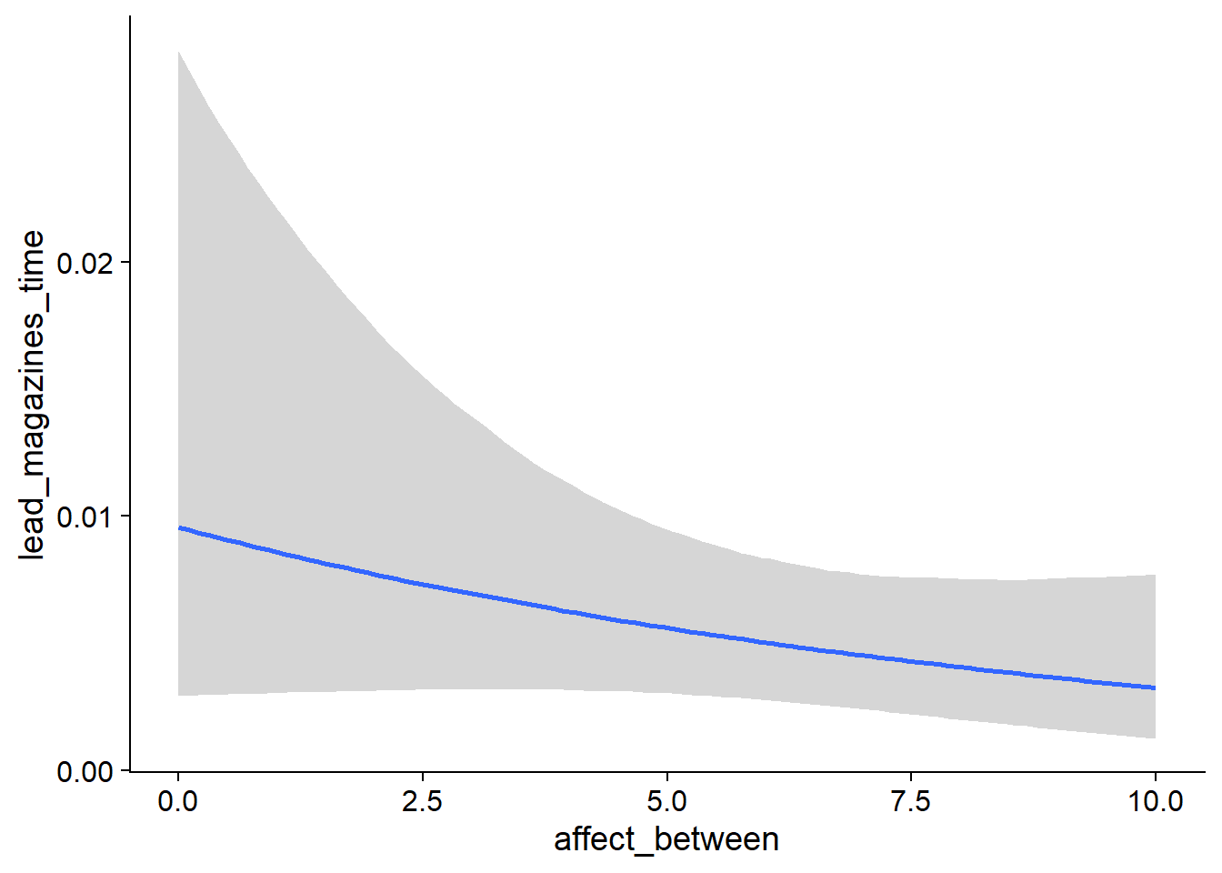
Figure 4.153: Conditional effects for Affect-Magazines model
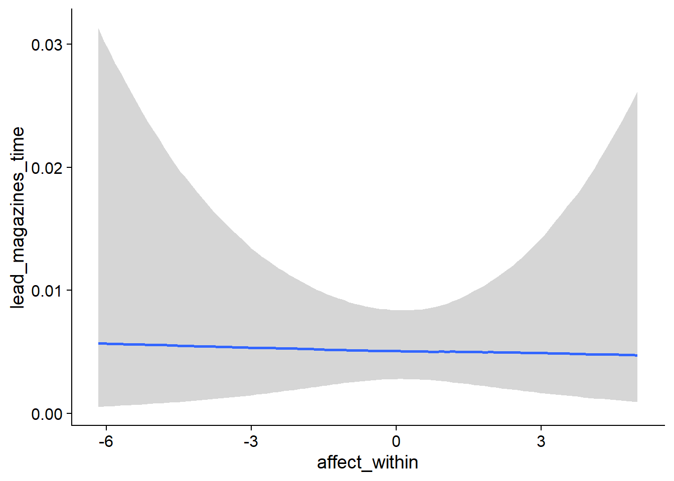
Figure 4.154: Conditional effects for Affect-Magazines model
##            used  (Mb) gc trigger   (Mb)  max used   (Mb)
## Ncells  3693724 197.3    6044351  322.9   6044351  322.9
## Vcells 23785727 181.5  193646602 1477.5 255811179 1951.7
4.7.2 Life satisfaction
4.7.2.1 Magazines on life satisfaction
magazines_life <-
  brm(
    data = working_file,
    family = gaussian,
    life_satisfaction ~
      1 +
      magazines_used_between +
      magazines_used_within +
      magazines_time_between +
      magazines_time_within +
      (1 +
         magazines_time_within +
         magazines_used_within
       | id),
    iter = 7000,
    warmup = 3000,
    chains = 4,
    cores = 4,
    seed = 42,
    control = list(adapt_delta = 0.95),
    file = here("models", "magazines_life")
  )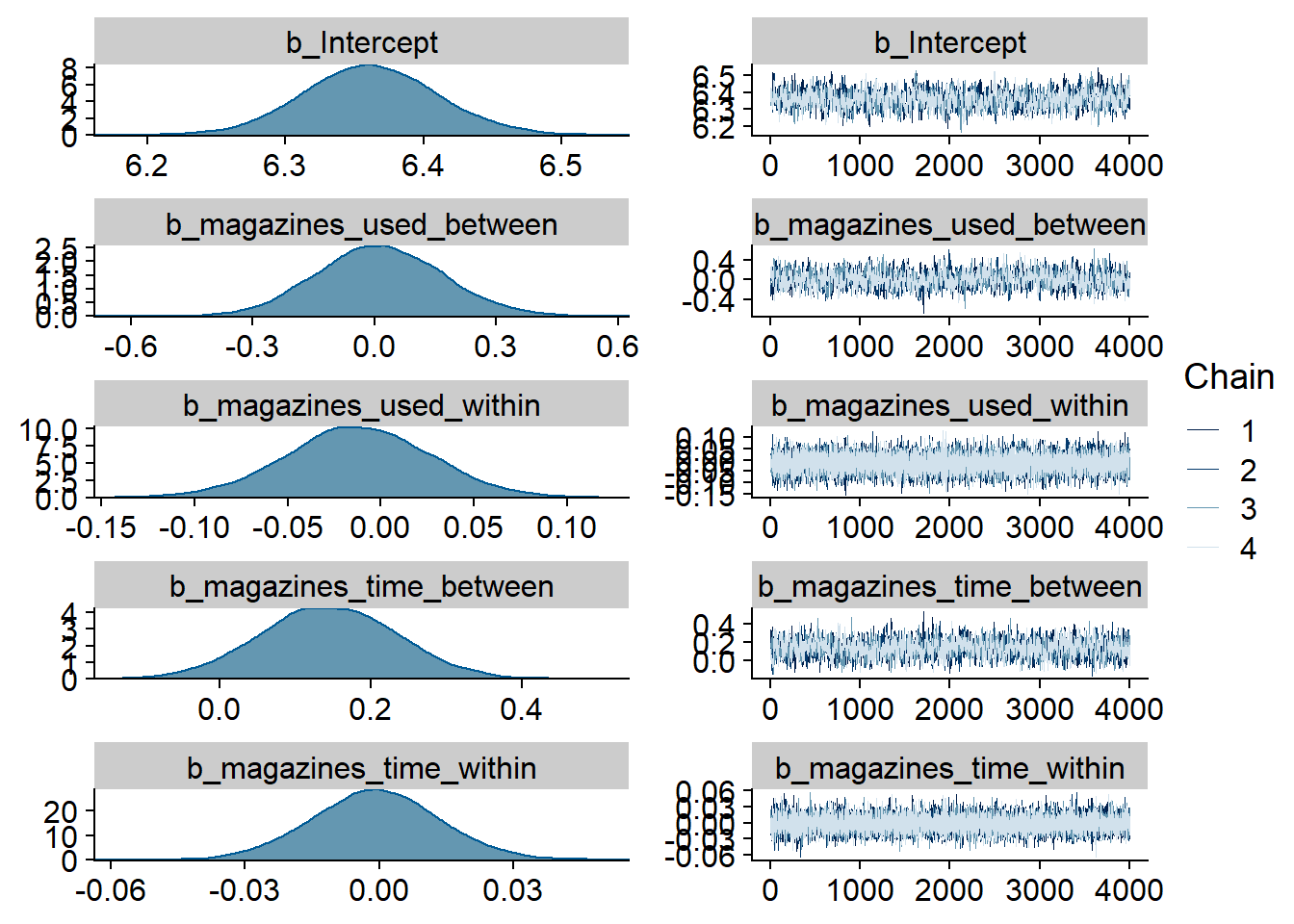
Figure 4.155: Traceplots and posterior distributions for Magazines-Life Satisfaction model
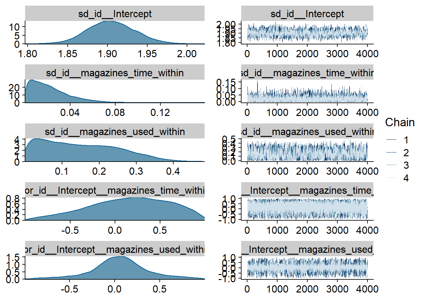
Figure 4.156: Traceplots and posterior distributions for Magazines-Life Satisfaction model
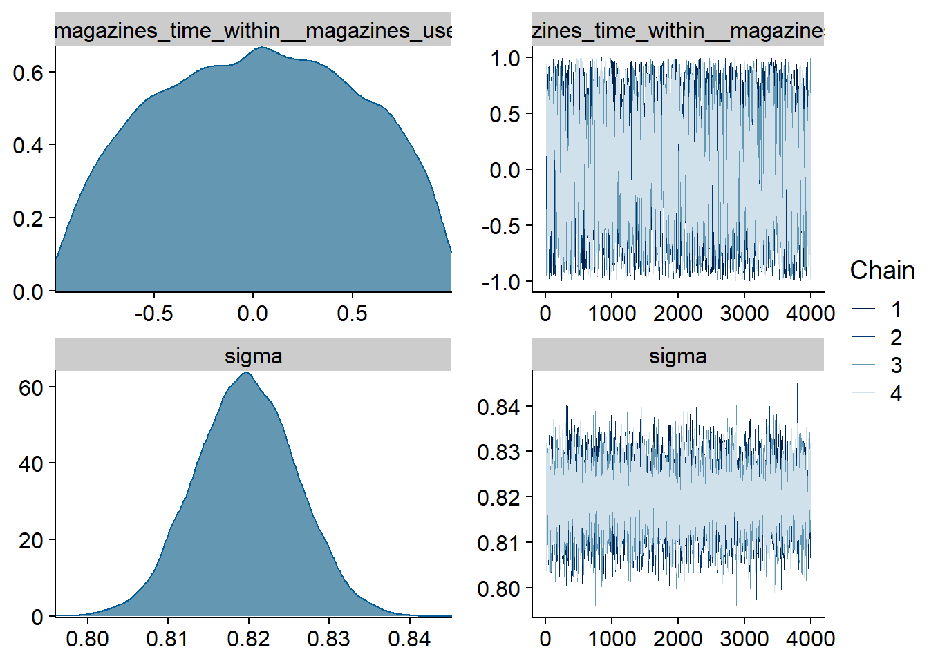
Figure 4.157: Traceplots and posterior distributions for Magazines-Life Satisfaction model
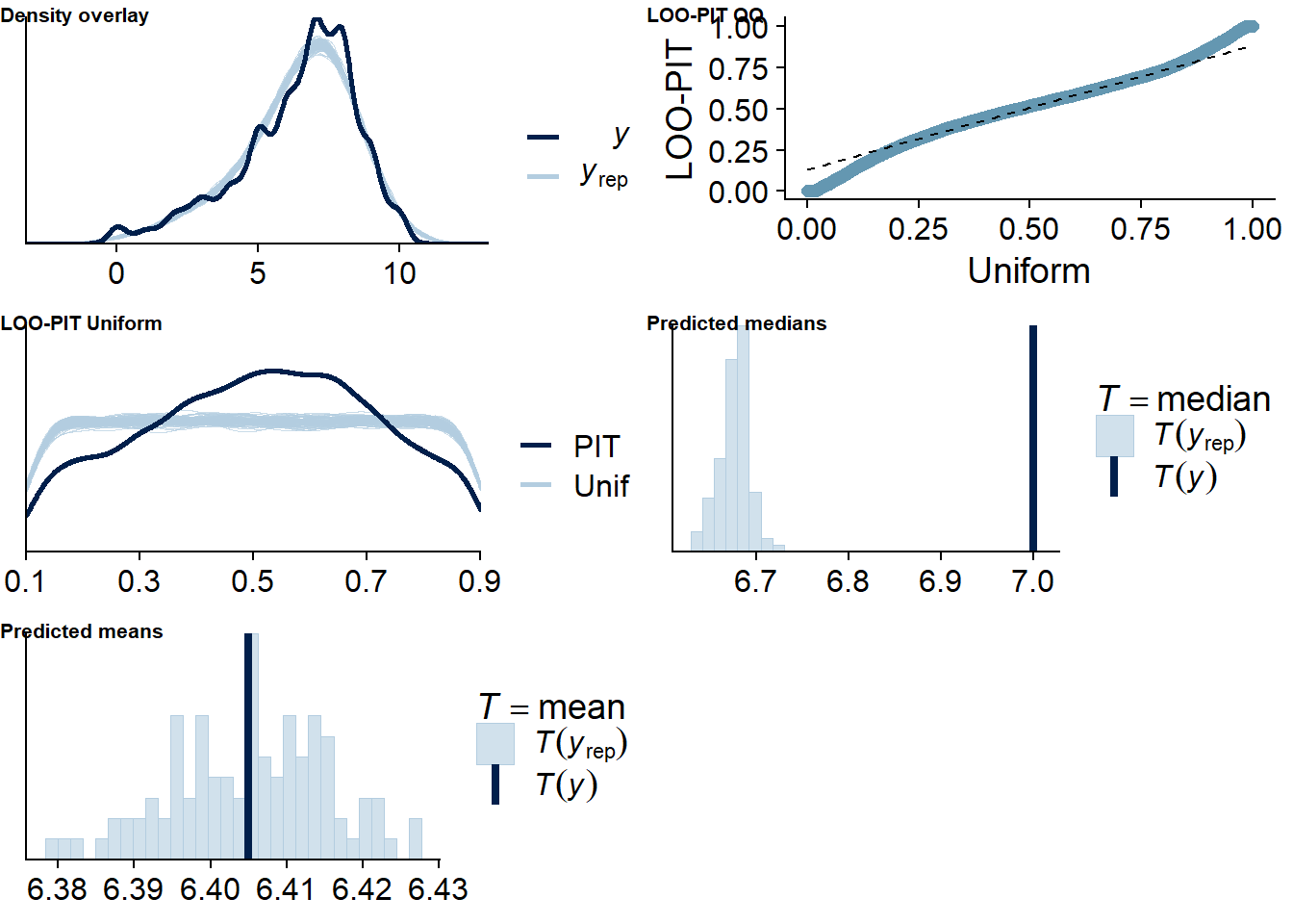
Figure 4.158: Posterior predictive checks for Magazines-Life Satisfaction model
The outliers are in about the same range as in previous models, and the model diagnostics look good.
magazines_life_loo <- loo(magazines_life)
magazines_life_loo
##
## Computed from 16000 by 10985 log-likelihood matrix
##
## Estimate SE
## elpd_loo -14595.4 146.5
## p_loo 2004.0 47.5
## looic 29190.8 293.0
## ------
## Monte Carlo SE of elpd_loo is NA.
##
## Pareto k diagnostic values:
## Count Pct. Min. n_eff
## (-Inf, 0.5] (good) 10612 96.6% 530
## (0.5, 0.7] (ok) 317 2.9% 93
## (0.7, 1] (bad) 48 0.4% 17
## (1, Inf) (very bad) 8 0.1% 2
## See help('pareto-k-diagnostic') for details.Below the summary.
summary(magazines_life)## Family: gaussian
## Links: mu = identity; sigma = identity
## Formula: life_satisfaction ~ 1 + magazines_used_between + magazines_used_within + magazines_time_between + magazines_time_within + (1 + magazines_time_within + magazines_used_within | id)
## Data: working_file (Number of observations: 10985)
## Samples: 4 chains, each with iter = 7000; warmup = 3000; thin = 1;
## total post-warmup samples = 16000
##
## Group-Level Effects:
## ~id (Number of levels: 2159)
## Estimate Est.Error l-95% CI u-95% CI Rhat Bulk_ESS Tail_ESS
## sd(Intercept) 1.90 0.03 1.85 1.96 1.00 1863 3954
## sd(magazines_time_within) 0.02 0.02 0.00 0.07 1.00 6375 9043
## sd(magazines_used_within) 0.15 0.10 0.01 0.35 1.00 1687 5158
## cor(Intercept,magazines_time_within) 0.16 0.44 -0.75 0.89 1.00 24099 11489
## cor(Intercept,magazines_used_within) 0.05 0.32 -0.67 0.75 1.00 14167 6508
## cor(magazines_time_within,magazines_used_within) 0.02 0.50 -0.87 0.89 1.00 3963 7545
##
## Population-Level Effects:
## Estimate Est.Error l-95% CI u-95% CI Rhat Bulk_ESS Tail_ESS
## Intercept 6.36 0.05 6.27 6.46 1.00 927 1729
## magazines_used_between 0.01 0.15 -0.28 0.32 1.01 1070 2314
## magazines_used_within -0.01 0.04 -0.09 0.06 1.00 31653 13180
## magazines_time_between 0.14 0.09 -0.03 0.32 1.00 1527 3032
## magazines_time_within -0.00 0.01 -0.03 0.03 1.00 24387 12511
##
## Family Specific Parameters:
## Estimate Est.Error l-95% CI u-95% CI Rhat Bulk_ESS Tail_ESS
## sigma 0.82 0.01 0.81 0.83 1.00 16100 12142
##
## Samples were drawn using sampling(NUTS). For each parameter, Bulk_ESS
## and Tail_ESS are effective sample size measures, and Rhat is the potential
## scale reduction factor on split chains (at convergence, Rhat = 1).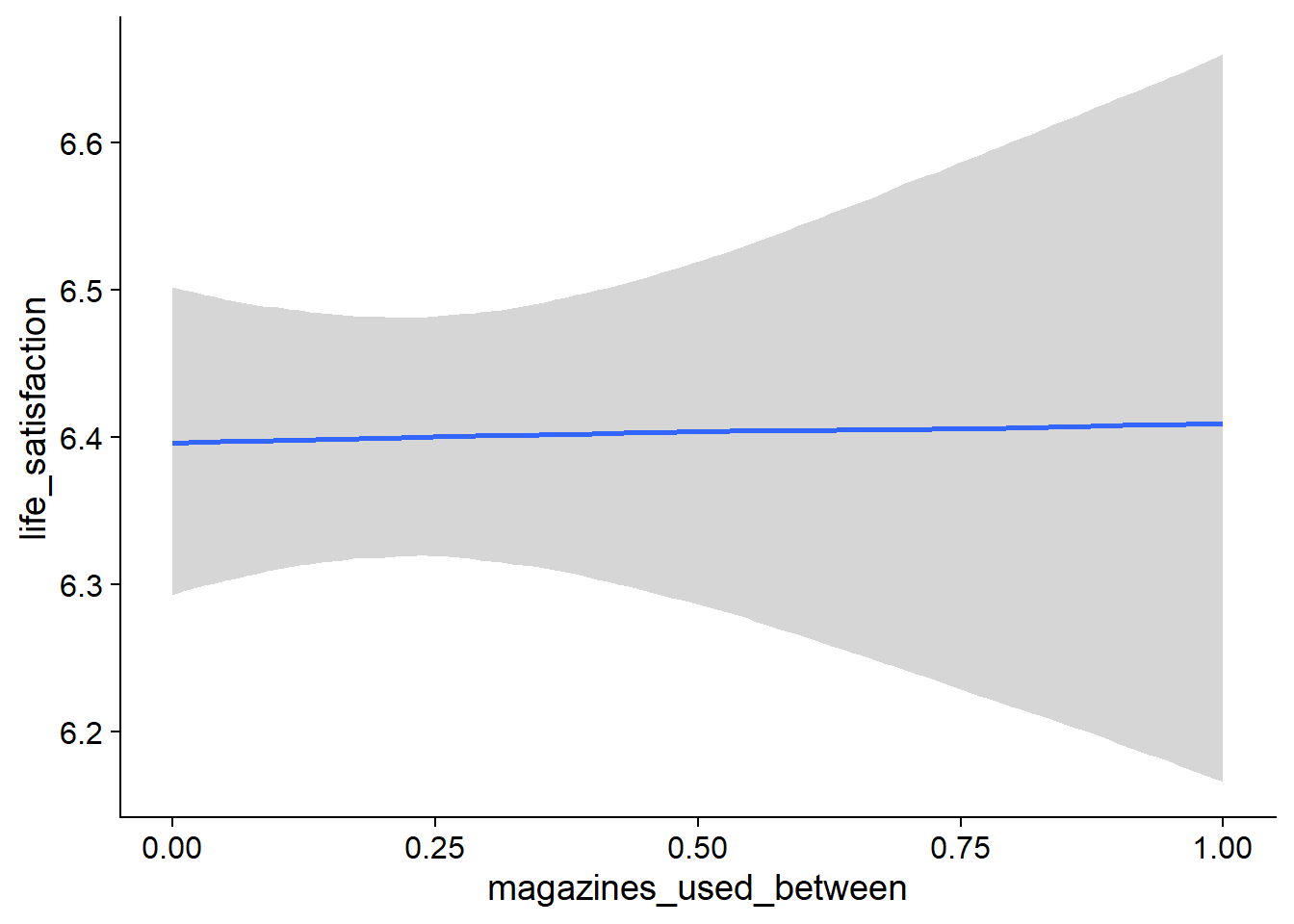
Figure 4.159: Conditional effects for Magazines-Life Satisfaction model
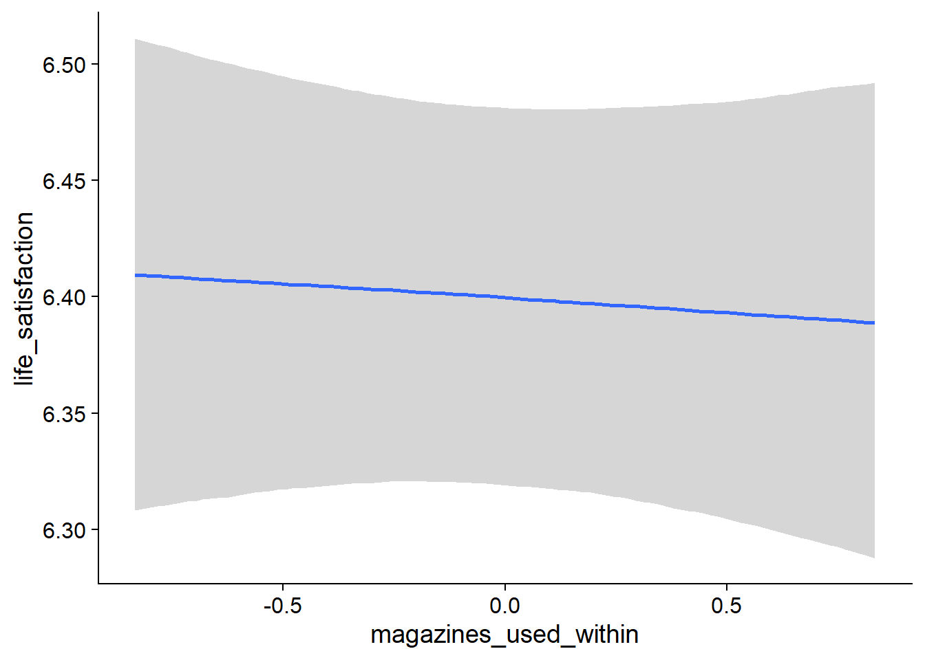
Figure 4.160: Conditional effects for Magazines-Life Satisfaction model
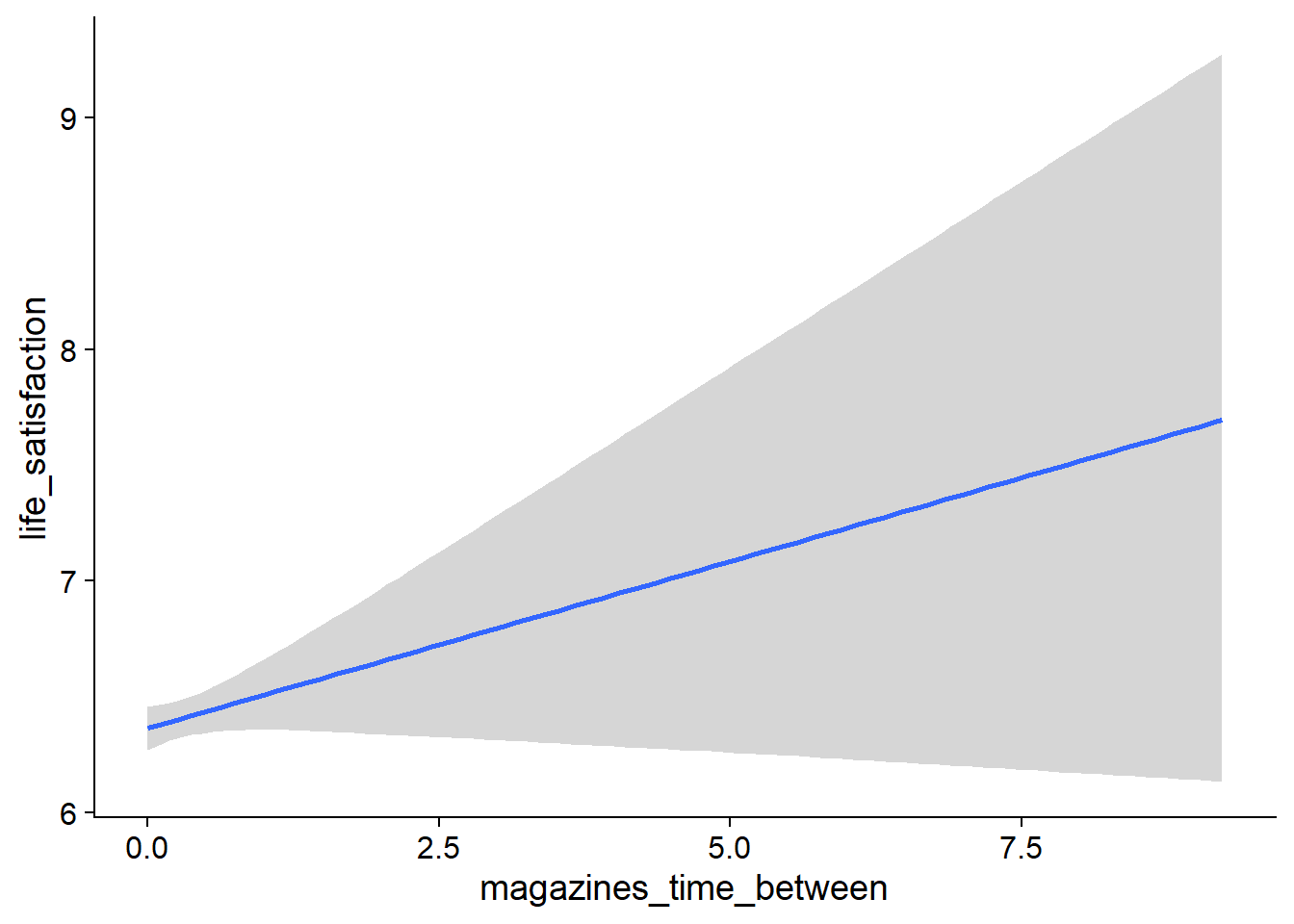
Figure 4.161: Conditional effects for Magazines-Life Satisfaction model
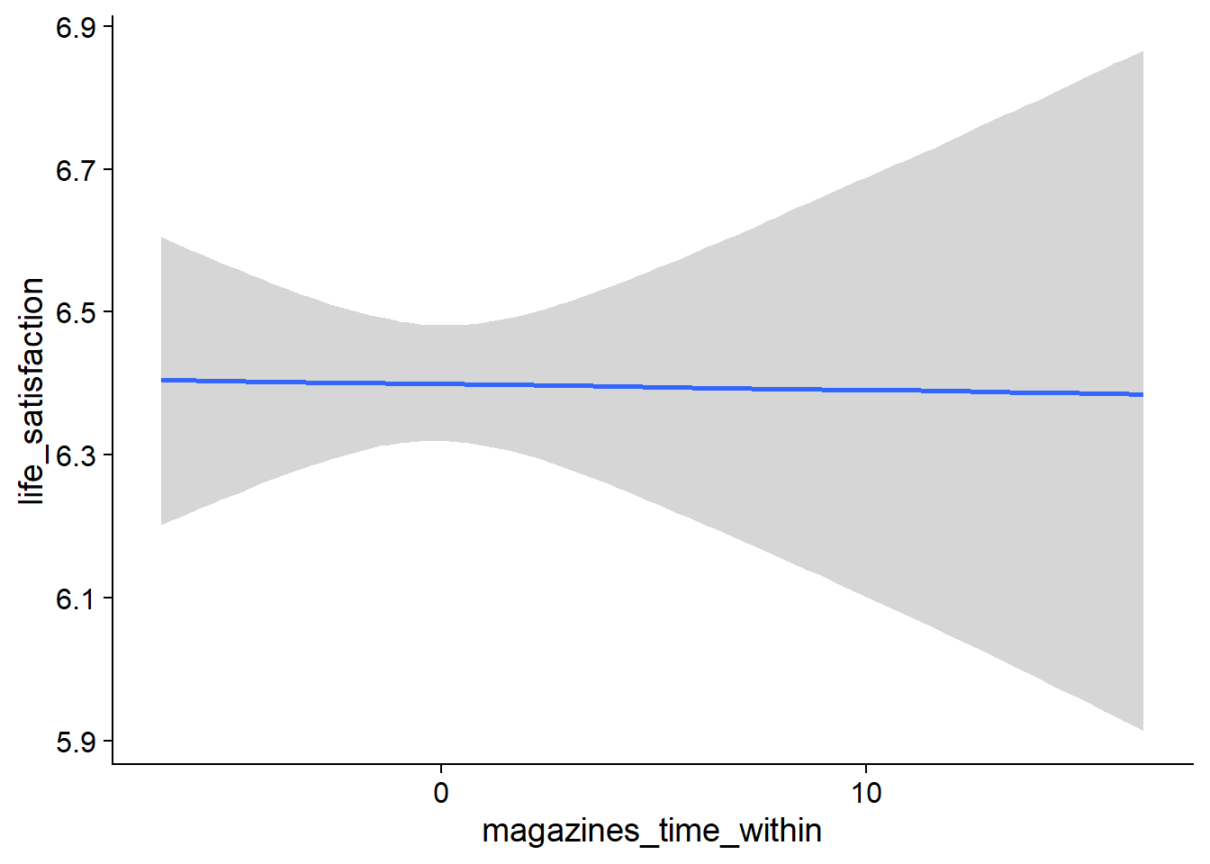
Figure 4.162: Conditional effects for Magazines-Life Satisfaction model
##            used  (Mb) gc trigger   (Mb)  max used   (Mb)
## Ncells  3693827 197.3    6044351  322.9   6044351  322.9
## Vcells 23786767 181.5  187577880 1431.2 255811179 1951.7
4.7.2.2 Life satisfaction on magazines
life_magazines <-
  brm(
    bf(
      # predicting continuous part
      lead_magazines_time ~
        1 +
        life_satisfaction_between +
        life_satisfaction_within +
        (1 +
           life_satisfaction_within
         | id),

      # predicting hurdle part
      hu ~
        1 +
        life_satisfaction_between +
        life_satisfaction_within +
        (1 +
           life_satisfaction_within
         | id)
    ),
    data = working_file,
    family = hurdle_gamma(),
    ,
    iter = 5000,
    warmup = 2000,
    chains = 4,
    cores = 4,
    seed = 42,
    control = list(adapt_delta = 0.95),
    file = here("models", "life_magazines")
  )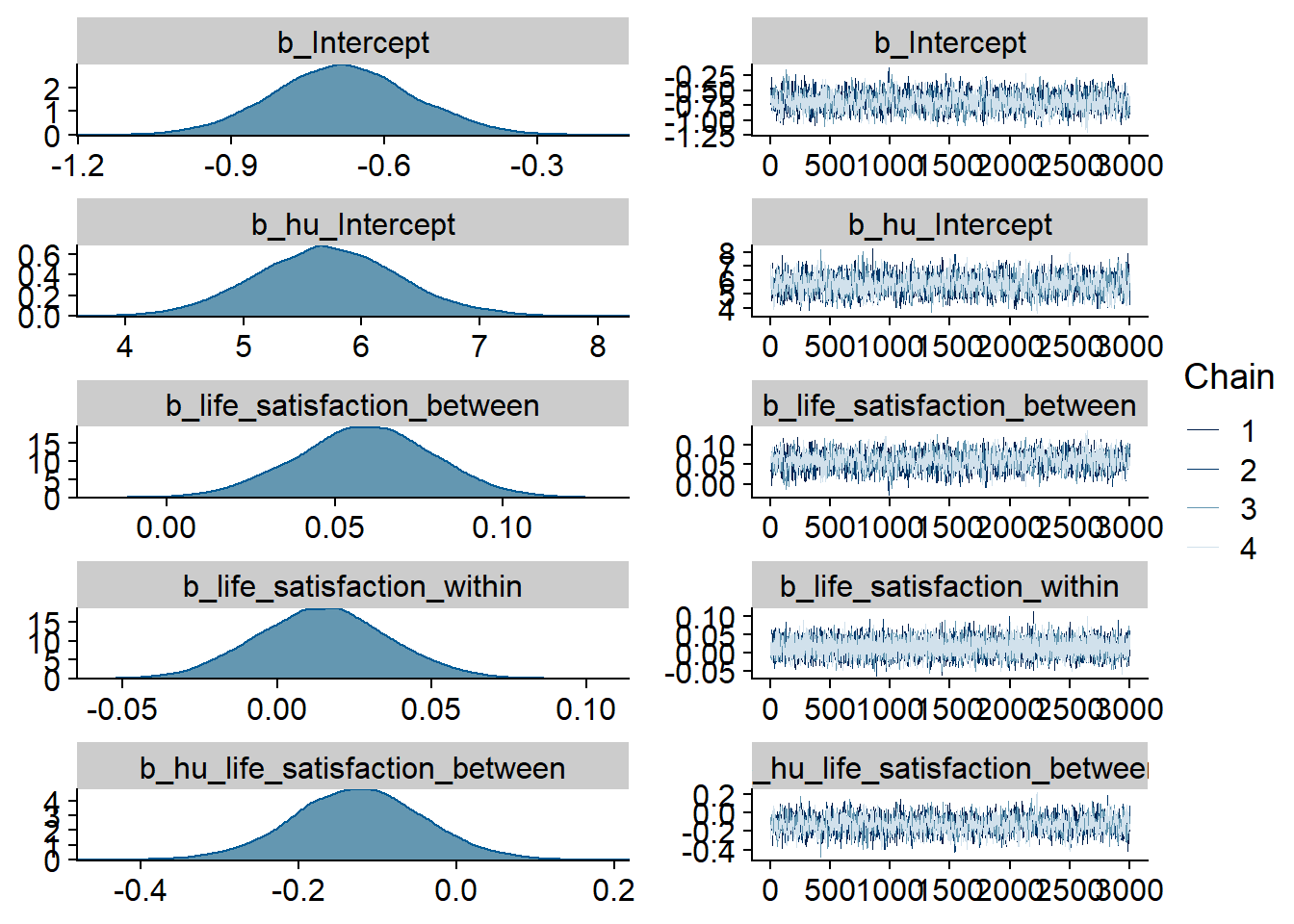
Figure 4.163: Traceplots and posterior distributions for Life Satisfaction-Magazines model
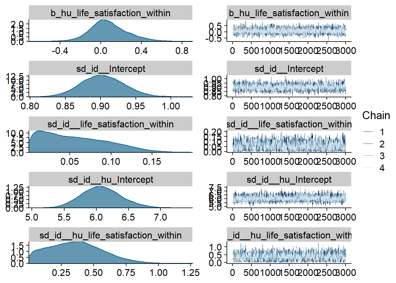
Figure 4.164: Traceplots and posterior distributions for Life Satisfaction-Magazines model
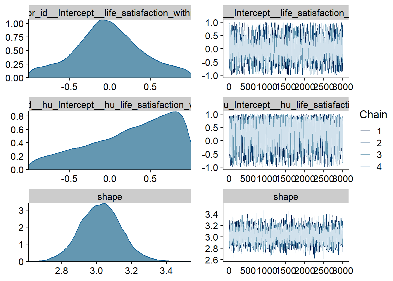
Figure 4.165: Traceplots and posterior distributions for Life Satisfaction-Magazines model
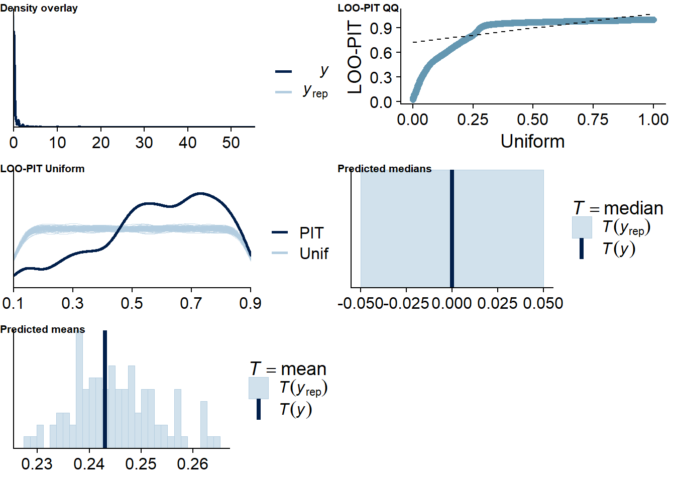
Figure 4.166: Posterior predictive checks for Life Satisfaction-Magazines model
There are more potentially influential values than in earlier models.
life_magazines_loo <- loo(life_magazines)
life_magazines_loo
##
## Computed from 12000 by 8698 log-likelihood matrix
##
## Estimate SE
## elpd_loo -3100.1 95.9
## p_loo 1249.2 45.0
## looic 6200.1 191.7
## ------
## Monte Carlo SE of elpd_loo is NA.
##
## Pareto k diagnostic values:
## Count Pct. Min. n_eff
## (-Inf, 0.5] (good) 7785 89.5% 786
## (0.5, 0.7] (ok) 596 6.9% 176
## (0.7, 1] (bad) 240 2.8% 20
## (1, Inf) (very bad) 77 0.9% 2
## See help('pareto-k-diagnostic') for details.Below the summary.
summary(life_magazines)## Family: hurdle_gamma
## Links: mu = log; shape = identity; hu = logit
## Formula: lead_magazines_time ~ 1 + life_satisfaction_between + life_satisfaction_within + (1 + life_satisfaction_within | id)
## hu ~ 1 + life_satisfaction_between + life_satisfaction_within + (1 + life_satisfaction_within | id)
## Data: working_file (Number of observations: 8698)
## Samples: 4 chains, each with iter = 5000; warmup = 2000; thin = 1;
## total post-warmup samples = 12000
##
## Group-Level Effects:
## ~id (Number of levels: 2157)
## Estimate Est.Error l-95% CI u-95% CI Rhat Bulk_ESS Tail_ESS
## sd(Intercept) 0.90 0.03 0.84 0.96 1.00 2141 4691
## sd(life_satisfaction_within) 0.06 0.04 0.00 0.14 1.00 1469 3379
## sd(hu_Intercept) 6.08 0.31 5.51 6.73 1.00 2408 5107
## sd(hu_life_satisfaction_within) 0.36 0.21 0.02 0.79 1.00 1554 2648
## cor(Intercept,life_satisfaction_within) -0.02 0.42 -0.86 0.85 1.00 7606 4536
## cor(hu_Intercept,hu_life_satisfaction_within) 0.27 0.51 -0.84 0.96 1.00 5198 5597
##
## Population-Level Effects:
## Estimate Est.Error l-95% CI u-95% CI Rhat Bulk_ESS Tail_ESS
## Intercept -0.68 0.14 -0.95 -0.41 1.00 1745 2929
## hu_Intercept 5.71 0.61 4.53 6.95 1.00 2106 4345
## life_satisfaction_between 0.06 0.02 0.02 0.10 1.00 1761 3200
## life_satisfaction_within 0.01 0.02 -0.03 0.06 1.00 10225 9627
## hu_life_satisfaction_between -0.12 0.08 -0.29 0.04 1.00 1915 3818
## hu_life_satisfaction_within 0.08 0.18 -0.26 0.48 1.00 4963 5944
##
## Family Specific Parameters:
## Estimate Est.Error l-95% CI u-95% CI Rhat Bulk_ESS Tail_ESS
## shape 3.02 0.12 2.80 3.25 1.00 7339 8694
##
## Samples were drawn using sampling(NUTS). For each parameter, Bulk_ESS
## and Tail_ESS are effective sample size measures, and Rhat is the potential
## scale reduction factor on split chains (at convergence, Rhat = 1).
Figure 4.167: Conditional effects for Life Satisfaction-Magazines model
Figure 4.168: Conditional effects for Life Satisfaction-Magazines model
##            used  (Mb) gc trigger   (Mb)  max used   (Mb)
## Ncells  3693951 197.3    6044351  322.9   6044351  322.9
## Vcells 23787805 181.5  181752182 1386.7 255811179 1951.7
4.8 Audiobooks
4.8.1 Affect
4.8.1.1 Audiobooks on affect
audiobooks_affect <-
  brm(
    data = working_file,
    family = gaussian,
    affect ~
      1 +
      audiobooks_used_between +
      audiobooks_used_within +
      audiobooks_time_between +
      audiobooks_time_within +
      (1 +
         audiobooks_time_within +
         audiobooks_used_within
       | id),
    iter = 7000,
    warmup = 3000,
    chains = 4,
    cores = 4,
    seed = 42,
    control = list(adapt_delta = 0.95),
    file = here("models", "audiobooks_affect")
  )
Figure 4.169: Traceplots and posterior distributions for Audiobooks-Affect model
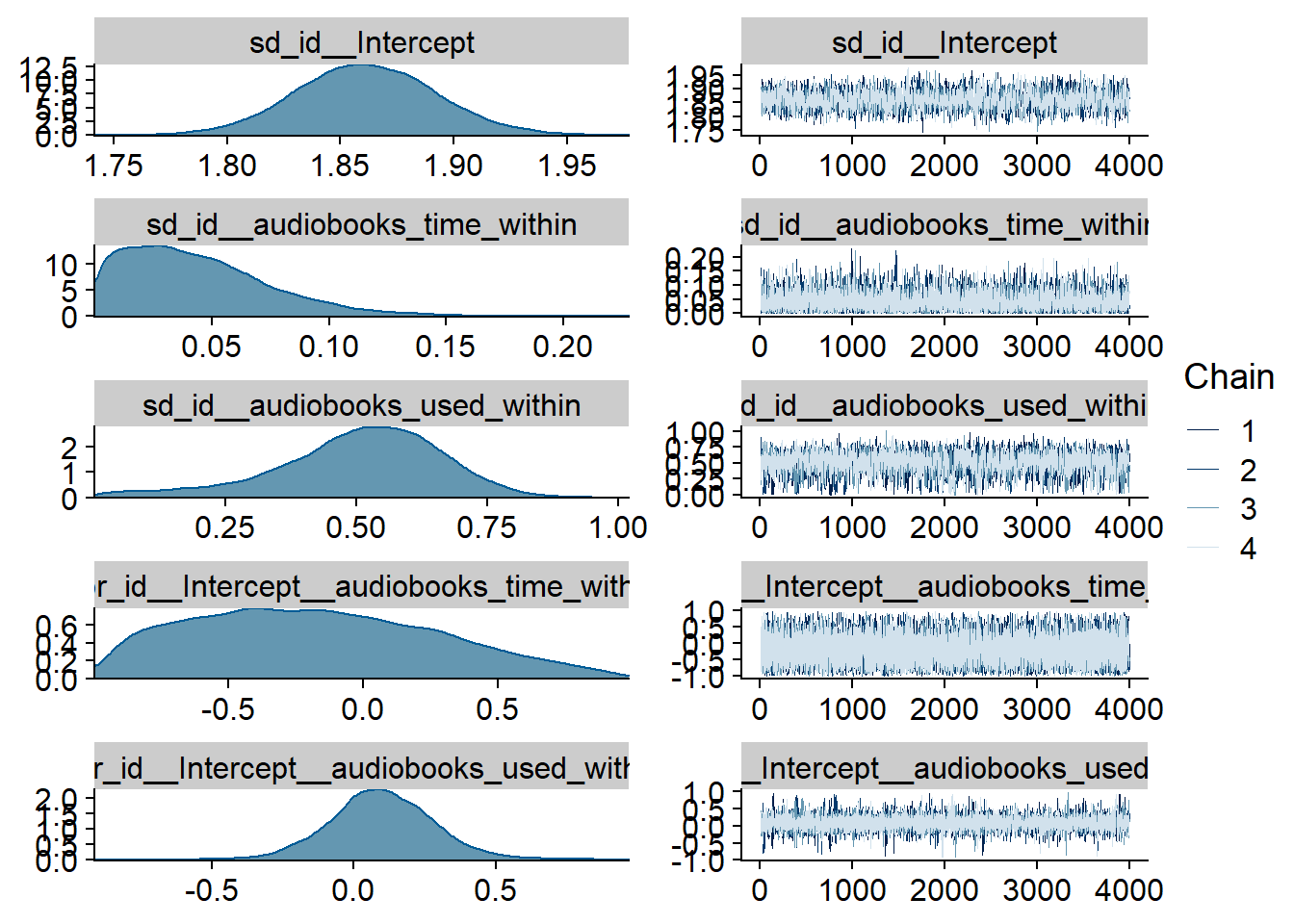
Figure 4.170: Traceplots and posterior distributions for Audiobooks-Affect model
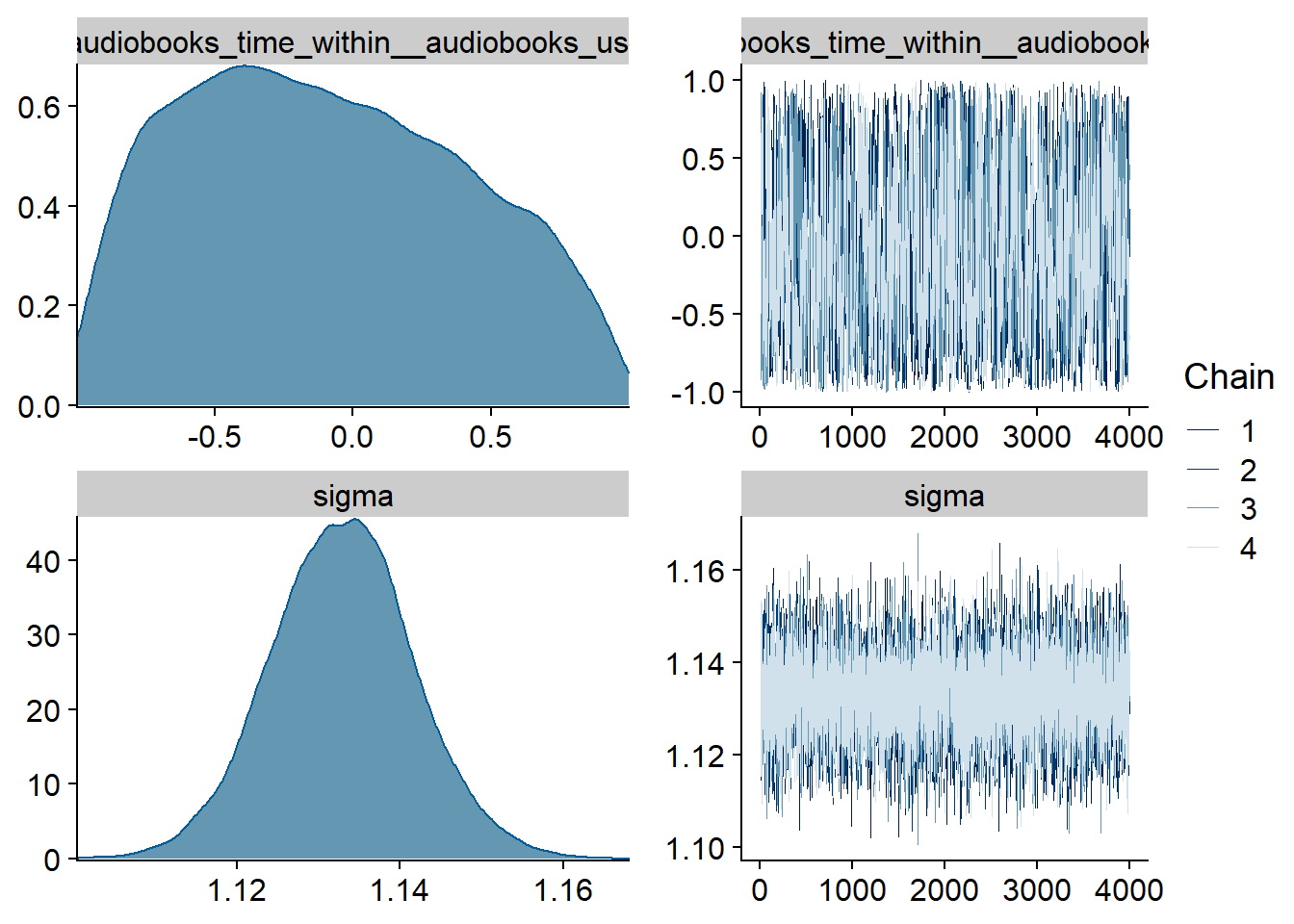
Figure 4.171: Traceplots and posterior distributions for Audiobooks-Affect model
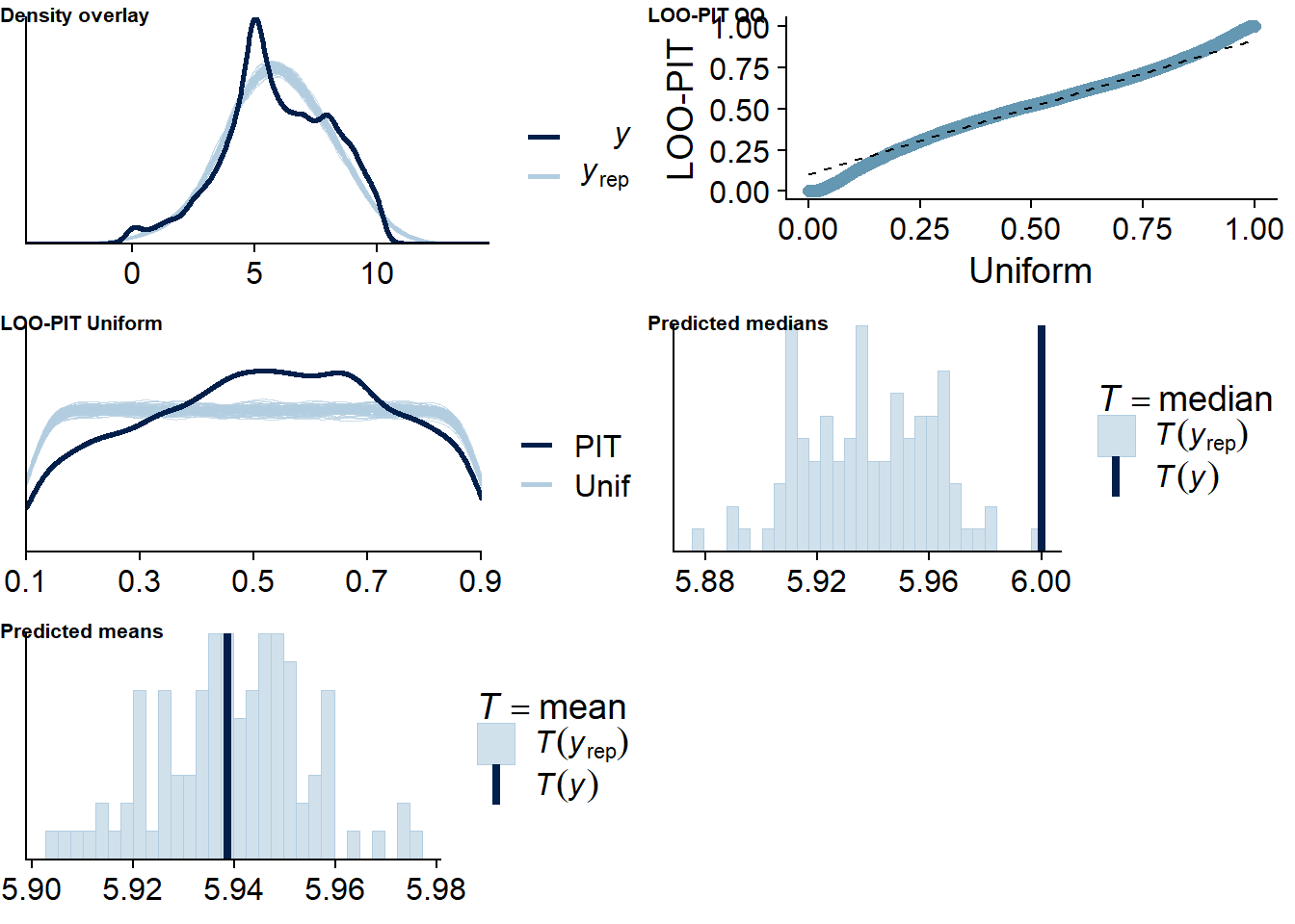
Figure 4.172: Posterior predictive checks for Audiobooks-Affect model
The outliers are in about the same range as in previous models, and the model diagnostics look good.
audiobooks_affect_loo <- loo(audiobooks_affect)
audiobooks_affect_loo
##
## Computed from 16000 by 10985 log-likelihood matrix
##
## Estimate SE
## elpd_loo -18111.9 105.6
## p_loo 1943.3 34.0
## looic 36223.8 211.3
## ------
## Monte Carlo SE of elpd_loo is NA.
##
## Pareto k diagnostic values:
## Count Pct. Min. n_eff
## (-Inf, 0.5] (good) 10617 96.6% 596
## (0.5, 0.7] (ok) 337 3.1% 134
## (0.7, 1] (bad) 31 0.3% 10
## (1, Inf) (very bad) 0 0.0% <NA>
## See help('pareto-k-diagnostic') for details.Below the summary.
summary(audiobooks_affect)## Family: gaussian
## Links: mu = identity; sigma = identity
## Formula: affect ~ 1 + audiobooks_used_between + audiobooks_used_within + audiobooks_time_between + audiobooks_time_within + (1 + audiobooks_time_within + audiobooks_used_within | id)
## Data: working_file (Number of observations: 10985)
## Samples: 4 chains, each with iter = 7000; warmup = 3000; thin = 1;
## total post-warmup samples = 16000
##
## Group-Level Effects:
## ~id (Number of levels: 2159)
## Estimate Est.Error l-95% CI u-95% CI Rhat Bulk_ESS Tail_ESS
## sd(Intercept) 1.86 0.03 1.80 1.92 1.00 2764 5234
## sd(audiobooks_time_within) 0.04 0.03 0.00 0.12 1.00 7055 7642
## sd(audiobooks_used_within) 0.50 0.16 0.11 0.77 1.00 1932 1603
## cor(Intercept,audiobooks_time_within) -0.18 0.45 -0.90 0.74 1.00 23390 11178
## cor(Intercept,audiobooks_used_within) 0.10 0.20 -0.27 0.49 1.00 11896 5089
## cor(audiobooks_time_within,audiobooks_used_within) -0.10 0.50 -0.91 0.85 1.01 1254 3605
##
## Population-Level Effects:
## Estimate Est.Error l-95% CI u-95% CI Rhat Bulk_ESS Tail_ESS
## Intercept 5.98 0.05 5.89 6.07 1.00 1675 3771
## audiobooks_used_between -0.39 0.24 -0.86 0.09 1.00 1963 3615
## audiobooks_used_within -0.14 0.08 -0.30 0.02 1.00 20473 13050
## audiobooks_time_between -0.09 0.10 -0.28 0.10 1.00 2236 4846
## audiobooks_time_within 0.01 0.03 -0.04 0.07 1.00 17227 12197
##
## Family Specific Parameters:
## Estimate Est.Error l-95% CI u-95% CI Rhat Bulk_ESS Tail_ESS
## sigma 1.13 0.01 1.12 1.15 1.00 14117 11394
##
## Samples were drawn using sampling(NUTS). For each parameter, Bulk_ESS
## and Tail_ESS are effective sample size measures, and Rhat is the potential
## scale reduction factor on split chains (at convergence, Rhat = 1).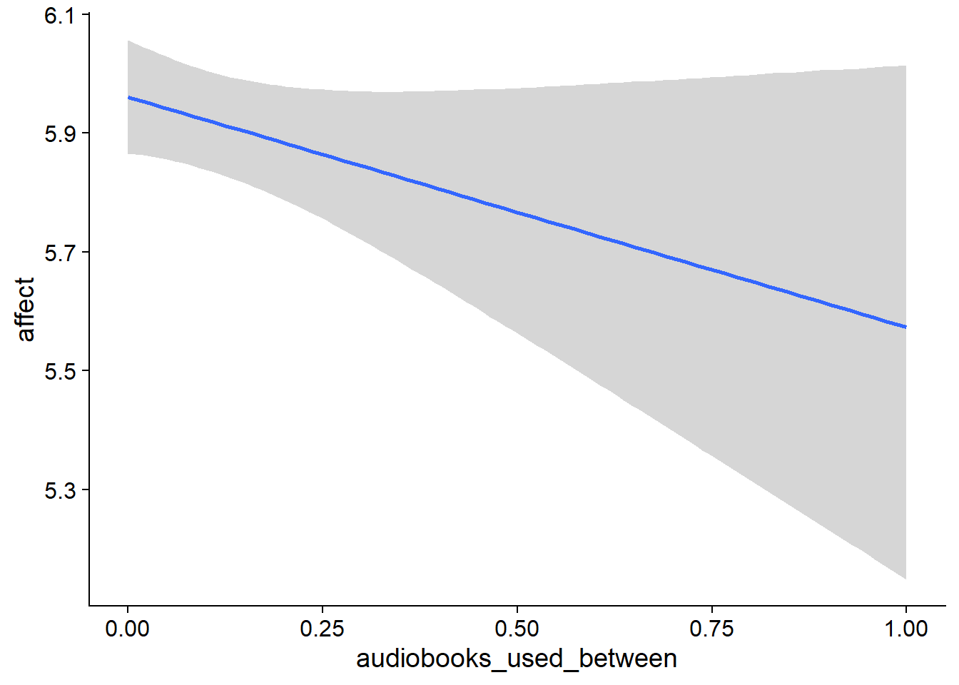
Figure 4.173: Conditional effects for Audiobooks-Affect model
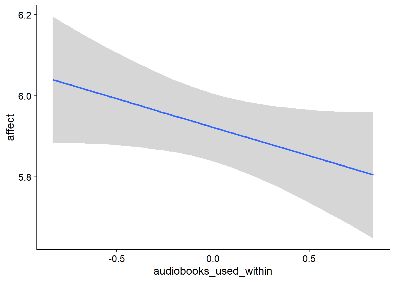
Figure 4.174: Conditional effects for Audiobooks-Affect model
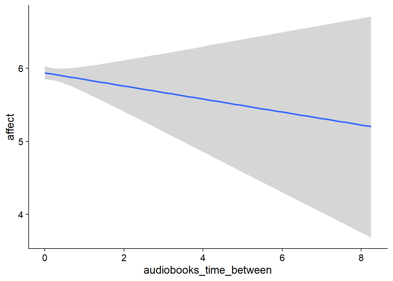
Figure 4.175: Conditional effects for Audiobooks-Affect model
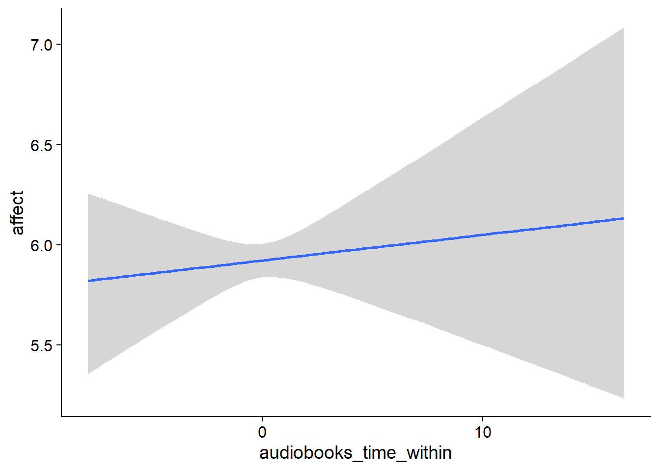
Figure 4.176: Conditional effects for Audiobooks-Affect model
##            used  (Mb) gc trigger   (Mb)  max used   (Mb)
## Ncells  3694054 197.3    6044351  322.9   6044351  322.9
## Vcells 23788824 181.5  176155817 1344.0 255811179 1951.7
4.8.1.2 Affect on audiobooks
affect_audiobooks <-
  brm(
    bf(
      # predicting continuous part
      lead_audiobooks_time ~
        1 +
        affect_between +
        affect_within +
        (1 +
           affect_within
         | id),

      # predicting hurdle part
      hu ~
        1 +
        affect_between +
        affect_within +
        (1 +
           affect_within
         | id)
    ),
    data = working_file,
    family = hurdle_gamma(),
    ,
    iter = 5000,
    warmup = 2000,
    chains = 4,
    cores = 4,
    seed = 42,
    control = list(adapt_delta = 0.95),
    file = here("models", "affect_audiobooks")
  )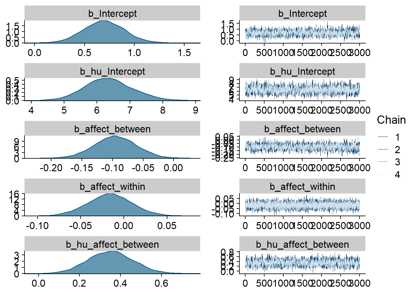
Figure 4.177: Traceplots and posterior distributions for Affect-Audiobooks model
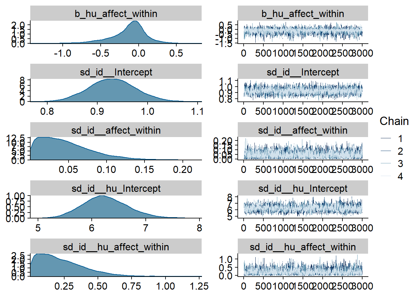
Figure 4.178: Traceplots and posterior distributions for Affect-Audiobooks model
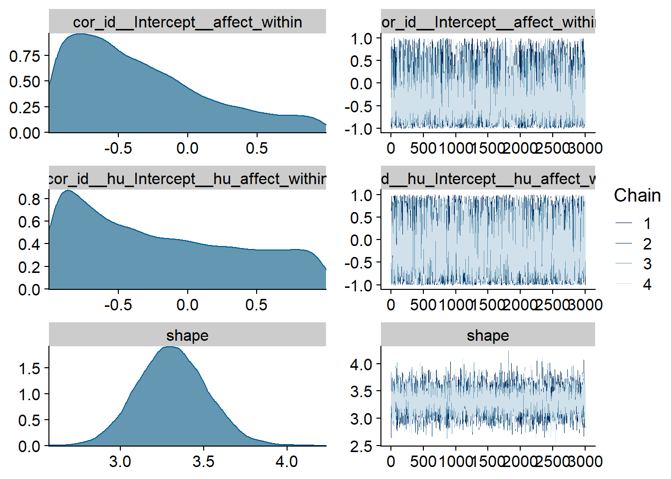
Figure 4.179: Traceplots and posterior distributions for Affect-Audiobooks model
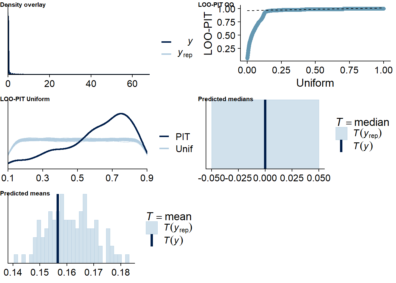
Figure 4.180: Posterior predictive checks for Affect-Audiobooks model
There are more potentially influential values than in earlier models.
affect_audiobooks_loo <- loo(affect_audiobooks)
affect_audiobooks_loo
##
## Computed from 12000 by 8698 log-likelihood matrix
##
## Estimate SE
## elpd_loo -1974.7 76.5
## p_loo 724.5 37.1
## looic 3949.5 152.9
## ------
## Monte Carlo SE of elpd_loo is NA.
##
## Pareto k diagnostic values:
## Count Pct. Min. n_eff
## (-Inf, 0.5] (good) 7816 89.9% 1415
## (0.5, 0.7] (ok) 673 7.7% 163
## (0.7, 1] (bad) 148 1.7% 18
## (1, Inf) (very bad) 61 0.7% 3
## See help('pareto-k-diagnostic') for details.Below the summary.
summary(affect_audiobooks)## Family: hurdle_gamma
## Links: mu = log; shape = identity; hu = logit
## Formula: lead_audiobooks_time ~ 1 + affect_between + affect_within + (1 + affect_within | id)
## hu ~ 1 + affect_between + affect_within + (1 + affect_within | id)
## Data: working_file (Number of observations: 8698)
## Samples: 4 chains, each with iter = 5000; warmup = 2000; thin = 1;
## total post-warmup samples = 12000
##
## Group-Level Effects:
## ~id (Number of levels: 2157)
## Estimate Est.Error l-95% CI u-95% CI Rhat Bulk_ESS Tail_ESS
## sd(Intercept) 0.93 0.05 0.84 1.02 1.00 2381 4767
## sd(affect_within) 0.05 0.03 0.00 0.13 1.00 2856 4443
## sd(hu_Intercept) 6.25 0.42 5.49 7.13 1.00 2026 4400
## sd(hu_affect_within) 0.23 0.17 0.01 0.63 1.00 2275 4840
## cor(Intercept,affect_within) -0.34 0.49 -0.97 0.83 1.00 8265 6872
## cor(hu_Intercept,hu_affect_within) -0.20 0.59 -0.98 0.92 1.00 4196 6420
##
## Population-Level Effects:
## Estimate Est.Error l-95% CI u-95% CI Rhat Bulk_ESS Tail_ESS
## Intercept 0.69 0.21 0.29 1.10 1.00 1906 3367
## hu_Intercept 6.36 0.75 4.95 7.89 1.00 2570 5020
## affect_between -0.10 0.03 -0.16 -0.03 1.00 1929 3515
## affect_within -0.02 0.03 -0.07 0.03 1.00 9563 8809
## hu_affect_between 0.35 0.11 0.14 0.57 1.00 2240 4669
## hu_affect_within -0.13 0.24 -0.70 0.28 1.00 3946 4560
##
## Family Specific Parameters:
## Estimate Est.Error l-95% CI u-95% CI Rhat Bulk_ESS Tail_ESS
## shape 3.31 0.21 2.91 3.72 1.00 5364 8173
##
## Samples were drawn using sampling(NUTS). For each parameter, Bulk_ESS
## and Tail_ESS are effective sample size measures, and Rhat is the potential
## scale reduction factor on split chains (at convergence, Rhat = 1).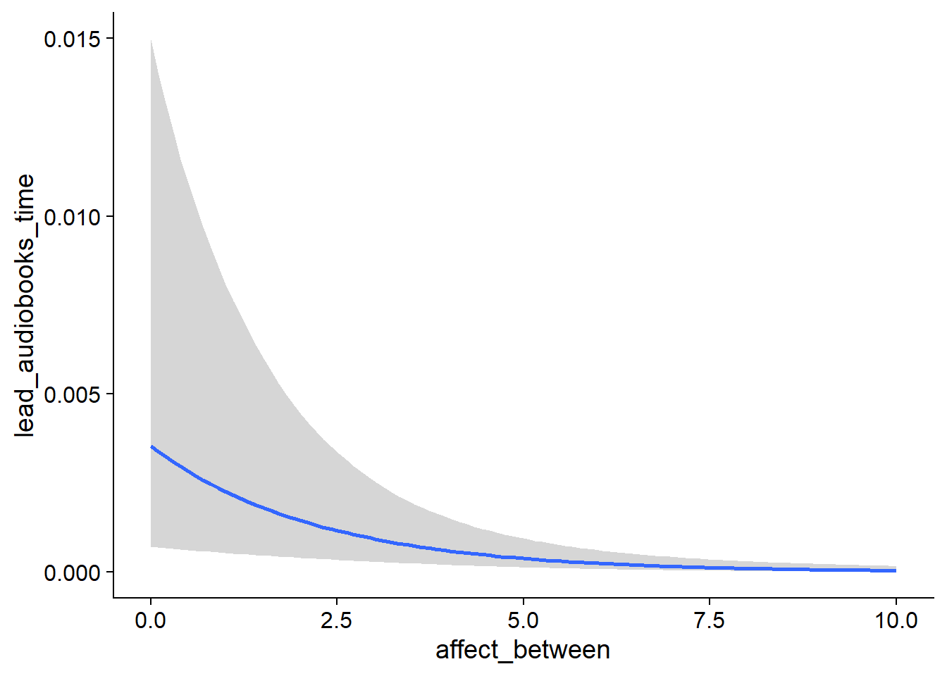
Figure 4.181: Conditional effects for Affect-Audiobooks model
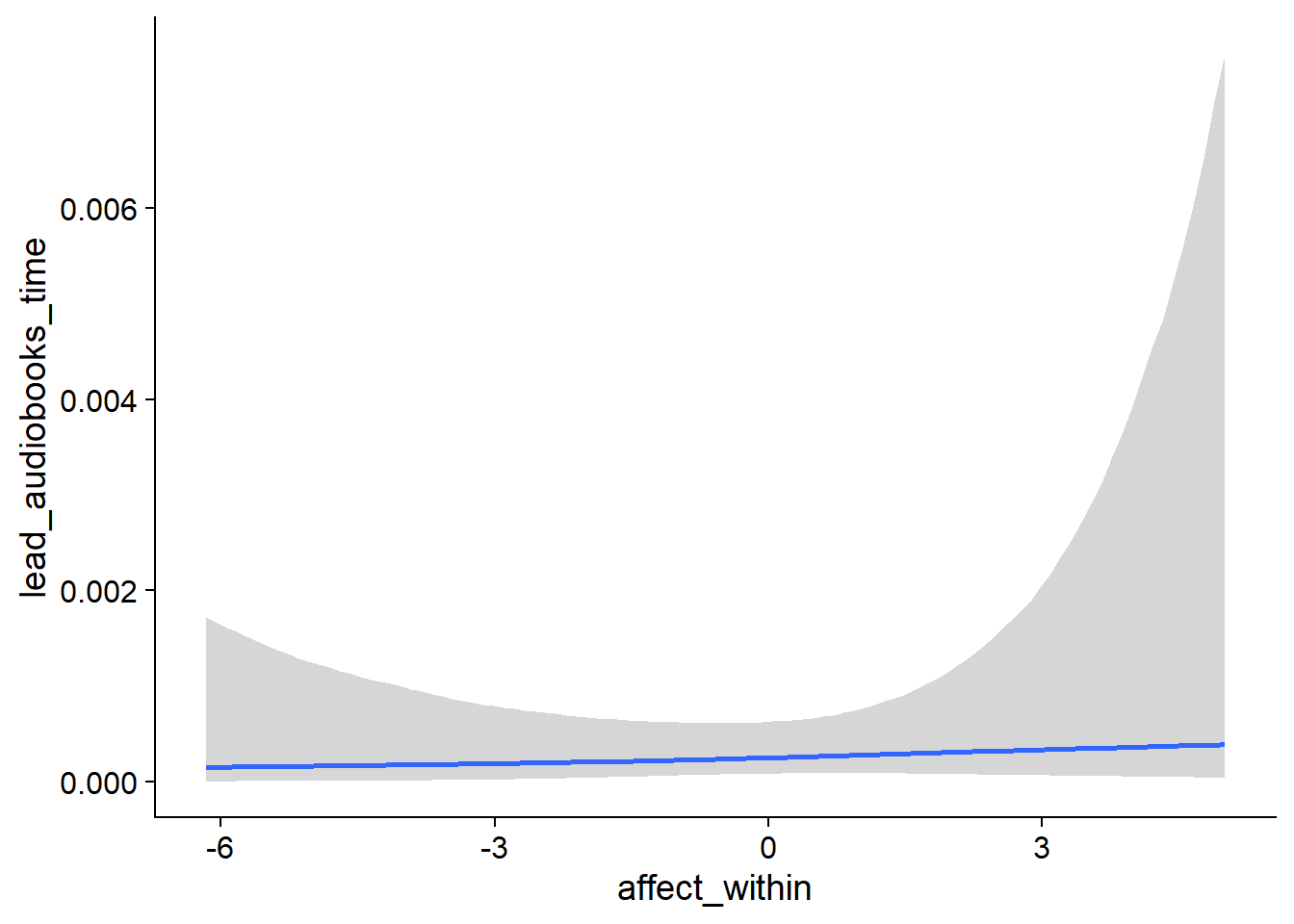
Figure 4.182: Conditional effects for Affect-Audiobooks model
##            used  (Mb) gc trigger   (Mb)  max used   (Mb)
## Ncells  3694154 197.3    6044351  322.9   6044351  322.9
## Vcells 23789779 181.6  170778996 1303.0 255811179 1951.7
4.8.2 Life satisfaction
4.8.2.1 Audiobooks on life satisfaction
audiobooks_life <-
  brm(
    data = working_file,
    family = gaussian,
    life_satisfaction ~
      1 +
      audiobooks_used_between +
      audiobooks_used_within +
      audiobooks_time_between +
      audiobooks_time_within +
      (1 +
         audiobooks_time_within +
         audiobooks_used_within
       | id),
    iter = 7000,
    warmup = 3000,
    chains = 4,
    cores = 4,
    seed = 42,
    control = list(adapt_delta = 0.95),
    file = here("models", "audiobooks_life")
  )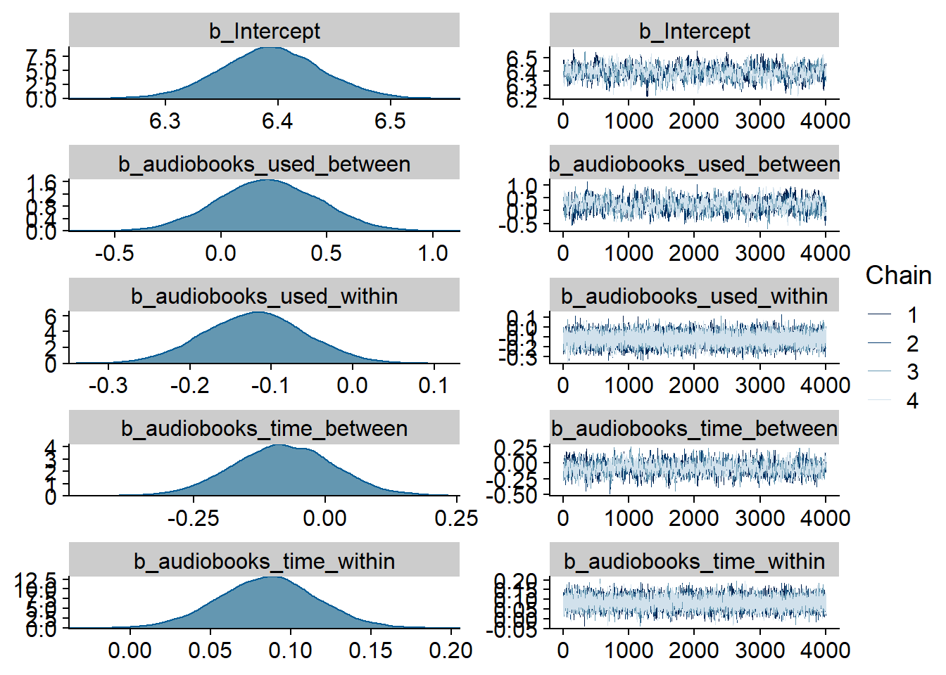
Figure 4.183: Traceplots and posterior distributions for Audiobooks-Life Satisfaction model
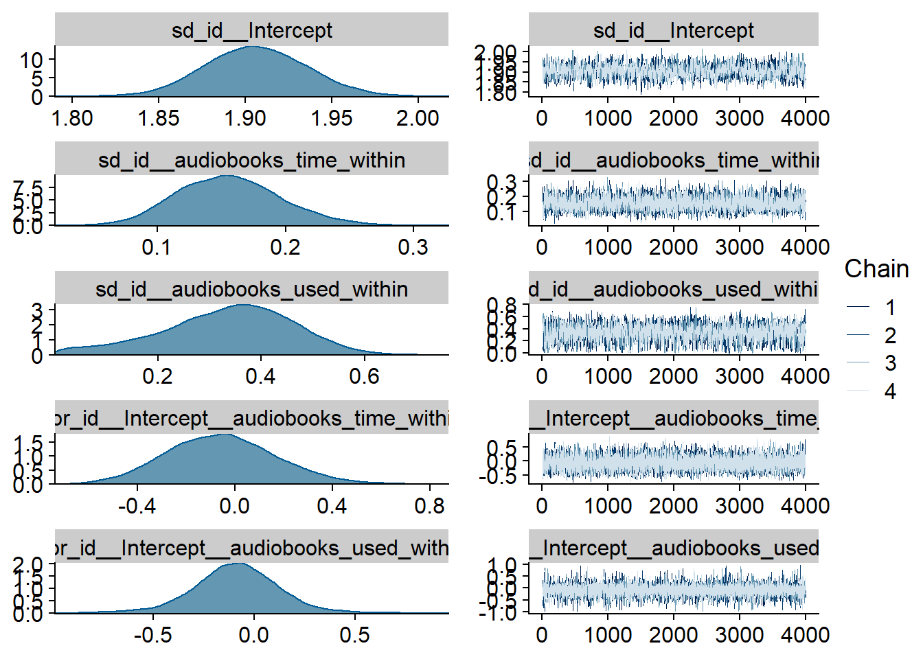
Figure 4.184: Traceplots and posterior distributions for Audiobooks-Life Satisfaction model
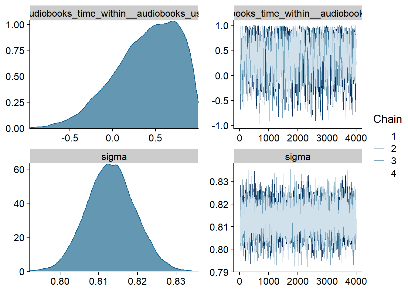
Figure 4.185: Traceplots and posterior distributions for Audiobooks-Life Satisfaction model
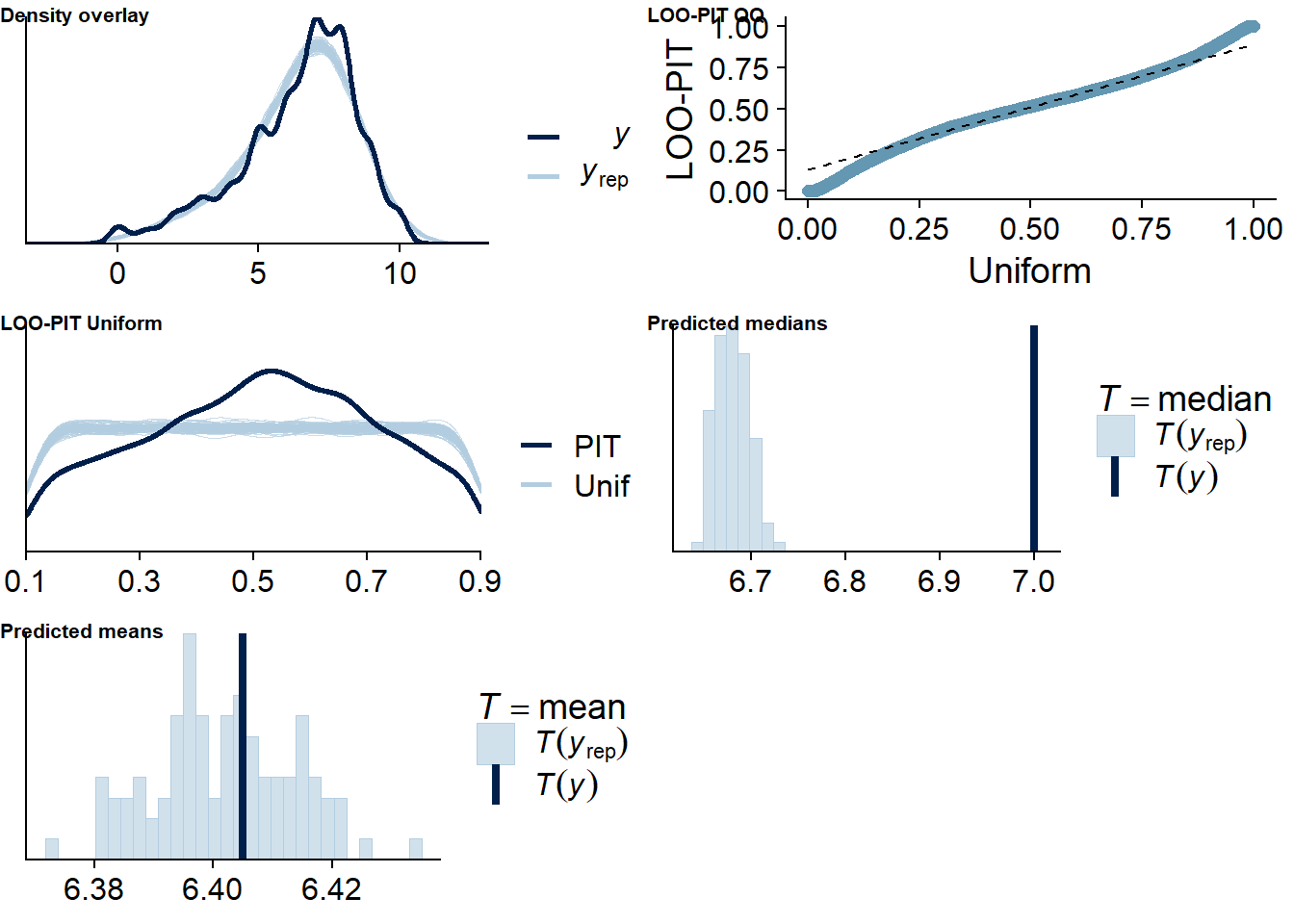
Figure 4.186: Posterior predictive checks for Audiobooks-Life Satisfaction model
The outliers are in about the same range as in previous models, and the model diagnostics look good.
audiobooks_life_loo <- loo(audiobooks_life)
audiobooks_life_loo
##
## Computed from 16000 by 10985 log-likelihood matrix
##
## Estimate SE
## elpd_loo -14563.4 146.4
## p_loo 2076.0 49.7
## looic 29126.7 292.7
## ------
## Monte Carlo SE of elpd_loo is NA.
##
## Pareto k diagnostic values:
## Count Pct. Min. n_eff
## (-Inf, 0.5] (good) 10494 95.5% 774
## (0.5, 0.7] (ok) 405 3.7% 130
## (0.7, 1] (bad) 75 0.7% 12
## (1, Inf) (very bad) 11 0.1% 4
## See help('pareto-k-diagnostic') for details.Below the summary.
summary(audiobooks_life)## Family: gaussian
## Links: mu = identity; sigma = identity
## Formula: life_satisfaction ~ 1 + audiobooks_used_between + audiobooks_used_within + audiobooks_time_between + audiobooks_time_within + (1 + audiobooks_time_within + audiobooks_used_within | id)
## Data: working_file (Number of observations: 10985)
## Samples: 4 chains, each with iter = 7000; warmup = 3000; thin = 1;
## total post-warmup samples = 16000
##
## Group-Level Effects:
## ~id (Number of levels: 2159)
## Estimate Est.Error l-95% CI u-95% CI Rhat Bulk_ESS Tail_ESS
## sd(Intercept) 1.91 0.03 1.85 1.96 1.00 1504 3385
## sd(audiobooks_time_within) 0.16 0.04 0.08 0.24 1.00 3754 7416
## sd(audiobooks_used_within) 0.33 0.13 0.05 0.55 1.00 1612 2250
## cor(Intercept,audiobooks_time_within) -0.06 0.22 -0.47 0.40 1.00 9935 9879
## cor(Intercept,audiobooks_used_within) -0.09 0.23 -0.56 0.36 1.00 9656 5194
## cor(audiobooks_time_within,audiobooks_used_within) 0.40 0.37 -0.43 0.94 1.00 1955 4210
##
## Population-Level Effects:
## Estimate Est.Error l-95% CI u-95% CI Rhat Bulk_ESS Tail_ESS
## Intercept 6.39 0.05 6.30 6.48 1.01 815 1490
## audiobooks_used_between 0.22 0.24 -0.24 0.69 1.01 820 1941
## audiobooks_used_within -0.12 0.06 -0.24 0.00 1.00 14105 12652
## audiobooks_time_between -0.08 0.10 -0.27 0.11 1.00 1154 2792
## audiobooks_time_within 0.09 0.03 0.02 0.15 1.00 9065 11633
##
## Family Specific Parameters:
## Estimate Est.Error l-95% CI u-95% CI Rhat Bulk_ESS Tail_ESS
## sigma 0.81 0.01 0.80 0.83 1.00 15476 12483
##
## Samples were drawn using sampling(NUTS). For each parameter, Bulk_ESS
## and Tail_ESS are effective sample size measures, and Rhat is the potential
## scale reduction factor on split chains (at convergence, Rhat = 1).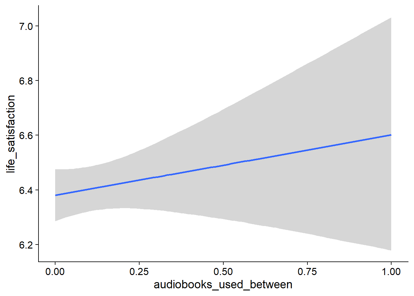
Figure 4.187: Conditional effects for Audiobooks-Life Satisfaction model
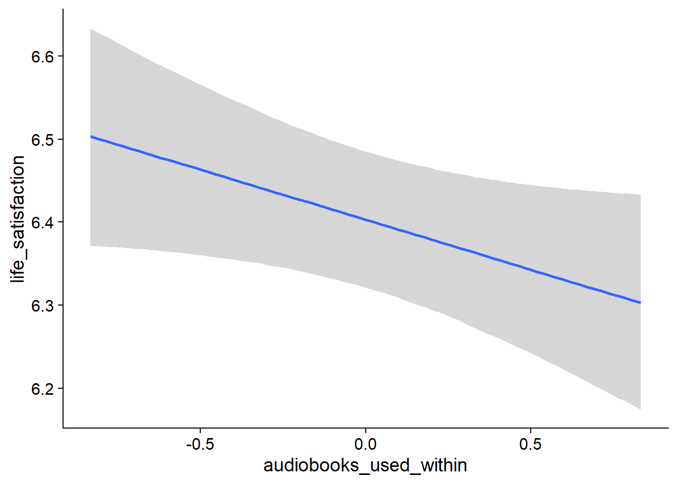
Figure 4.188: Conditional effects for Audiobooks-Life Satisfaction model
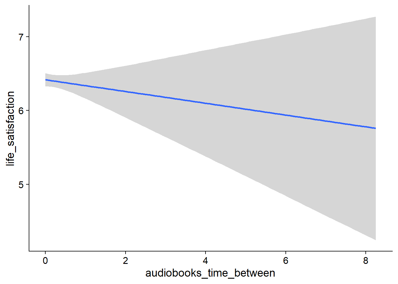
Figure 4.189: Conditional effects for Audiobooks-Life Satisfaction model
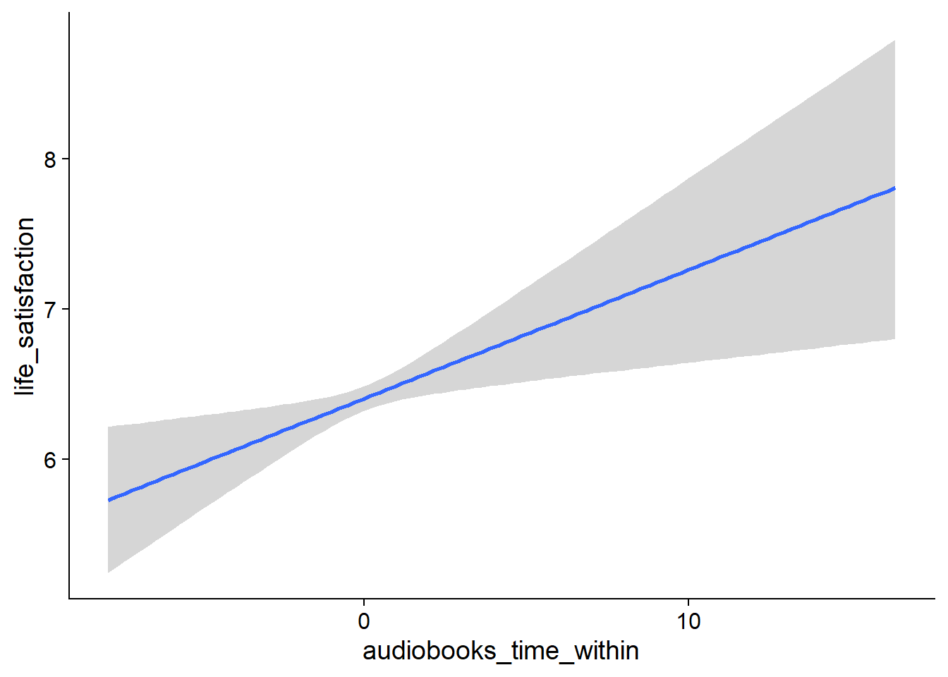
Figure 4.190: Conditional effects for Audiobooks-Life Satisfaction model
##            used  (Mb) gc trigger   (Mb)  max used   (Mb)
## Ncells  3694248 197.3    6044351  322.9   6044351  322.9
## Vcells 23790805 181.6  200236504 1527.7 255811179 1951.7
4.8.2.2 Life satisfaction on audiobooks
life_audiobooks <-
  brm(
    bf(
      # predicting continuous part
      lead_audiobooks_time ~
        1 +
        life_satisfaction_between +
        life_satisfaction_within +
        (1 +
           life_satisfaction_within
         | id),

      # predicting hurdle part
      hu ~
        1 +
        life_satisfaction_between +
        life_satisfaction_within +
        (1 +
           life_satisfaction_within
         | id)
    ),
    data = working_file,
    family = hurdle_gamma(),
    ,
    iter = 5000,
    warmup = 2000,
    chains = 4,
    cores = 4,
    seed = 42,
    control = list(adapt_delta = 0.95),
    file = here("models", "life_audiobooks")
  )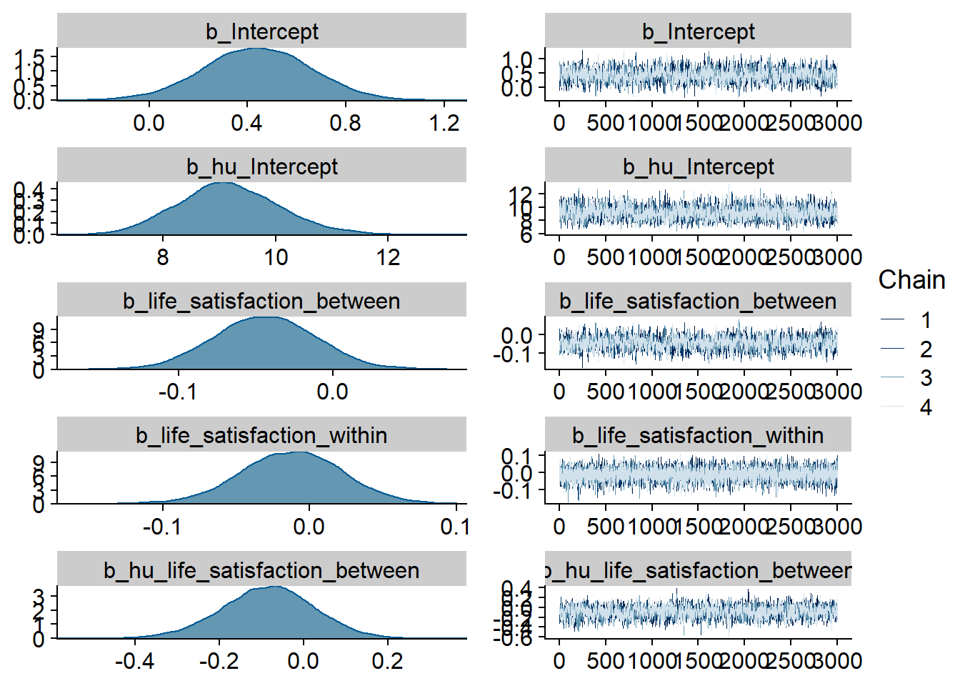
Figure 4.191: Traceplots and posterior distributions for Life Satisfaction-Audiobooks model
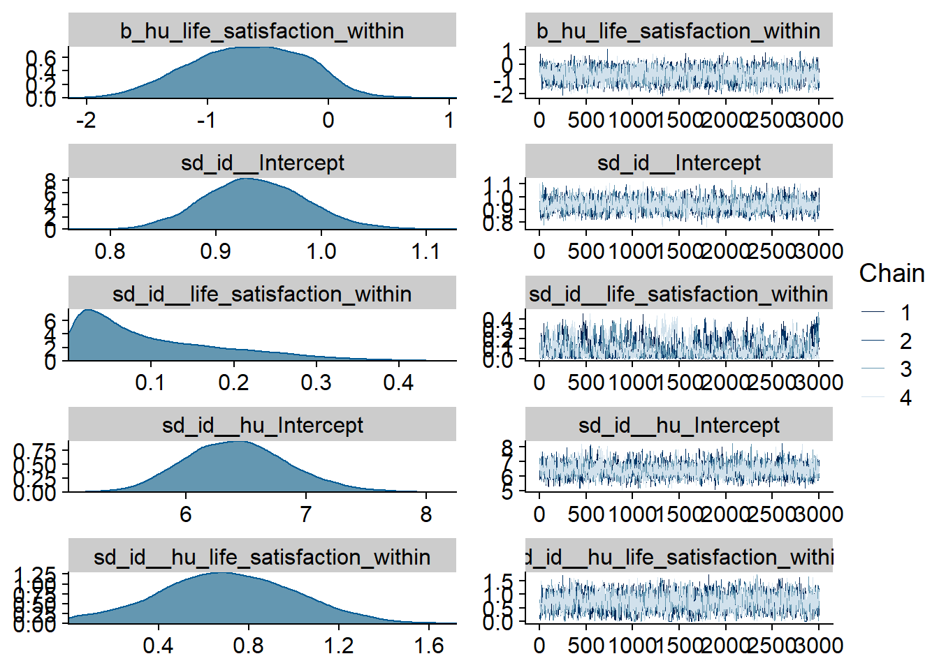
Figure 4.192: Traceplots and posterior distributions for Life Satisfaction-Audiobooks model
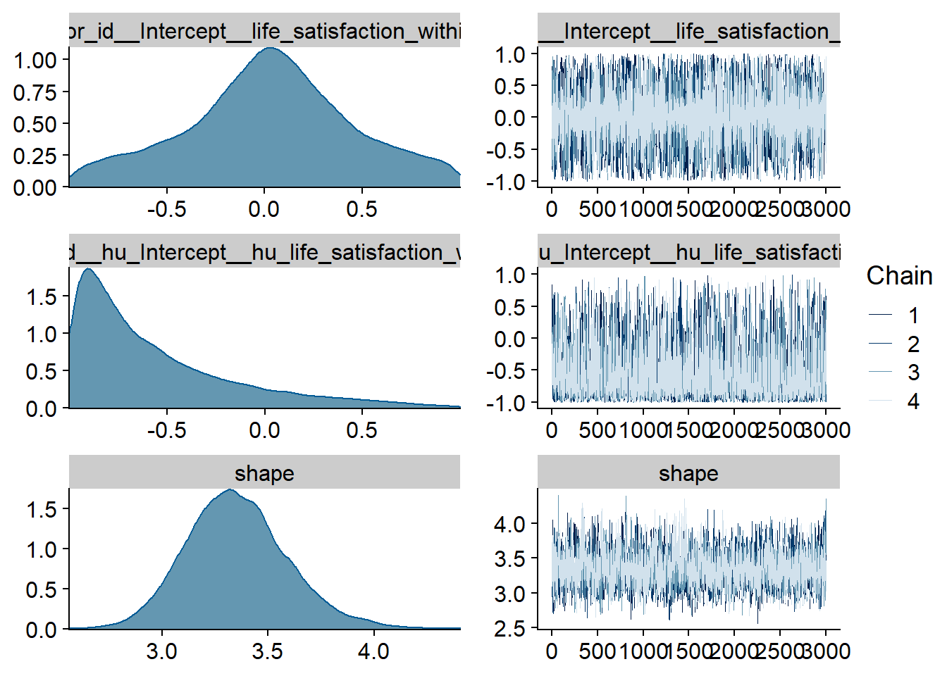
Figure 4.193: Traceplots and posterior distributions for Life Satisfaction-Audiobooks model

Figure 4.194: Posterior predictive checks for Life Satisfaction-Audiobooks model
There are more potentially influential values than in earlier models.
life_audiobooks_loo <- loo(life_audiobooks)
life_audiobooks_loo
##
## Computed from 12000 by 8698 log-likelihood matrix
##
## Estimate SE
## elpd_loo -1976.3 76.8
## p_loo 752.1 38.6
## looic 3952.6 153.6
## ------
## Monte Carlo SE of elpd_loo is NA.
##
## Pareto k diagnostic values:
## Count Pct. Min. n_eff
## (-Inf, 0.5] (good) 7550 86.8% 201
## (0.5, 0.7] (ok) 890 10.2% 225
## (0.7, 1] (bad) 191 2.2% 15
## (1, Inf) (very bad) 67 0.8% 2
## See help('pareto-k-diagnostic') for details.Below the summary.
summary(life_audiobooks)## Family: hurdle_gamma
## Links: mu = log; shape = identity; hu = logit
## Formula: lead_audiobooks_time ~ 1 + life_satisfaction_between + life_satisfaction_within + (1 + life_satisfaction_within | id)
## hu ~ 1 + life_satisfaction_between + life_satisfaction_within + (1 + life_satisfaction_within | id)
## Data: working_file (Number of observations: 8698)
## Samples: 4 chains, each with iter = 5000; warmup = 2000; thin = 1;
## total post-warmup samples = 12000
##
## Group-Level Effects:
## ~id (Number of levels: 2157)
## Estimate Est.Error l-95% CI u-95% CI Rhat Bulk_ESS Tail_ESS
## sd(Intercept) 0.94 0.05 0.85 1.04 1.00 2219 4037
## sd(life_satisfaction_within) 0.10 0.09 0.00 0.31 1.01 575 777
## sd(hu_Intercept) 6.43 0.43 5.64 7.33 1.00 1970 4389
## sd(hu_life_satisfaction_within) 0.70 0.30 0.11 1.30 1.00 1861 1620
## cor(Intercept,life_satisfaction_within) 0.03 0.43 -0.85 0.87 1.00 7258 5674
## cor(hu_Intercept,hu_life_satisfaction_within) -0.57 0.41 -0.99 0.53 1.00 2779 4482
##
## Population-Level Effects:
## Estimate Est.Error l-95% CI u-95% CI Rhat Bulk_ESS Tail_ESS
## Intercept 0.44 0.22 0.00 0.86 1.00 1454 2778
## hu_Intercept 9.17 0.91 7.48 11.07 1.00 2031 4155
## life_satisfaction_between -0.04 0.03 -0.11 0.02 1.00 1384 2656
## life_satisfaction_within -0.01 0.03 -0.08 0.06 1.00 6431 6701
## hu_life_satisfaction_between -0.09 0.11 -0.31 0.12 1.00 1958 3828
## hu_life_satisfaction_within -0.67 0.47 -1.58 0.17 1.00 2648 6084
##
## Family Specific Parameters:
## Estimate Est.Error l-95% CI u-95% CI Rhat Bulk_ESS Tail_ESS
## shape 3.35 0.24 2.92 3.87 1.00 1802 2466
##
## Samples were drawn using sampling(NUTS). For each parameter, Bulk_ESS
## and Tail_ESS are effective sample size measures, and Rhat is the potential
## scale reduction factor on split chains (at convergence, Rhat = 1).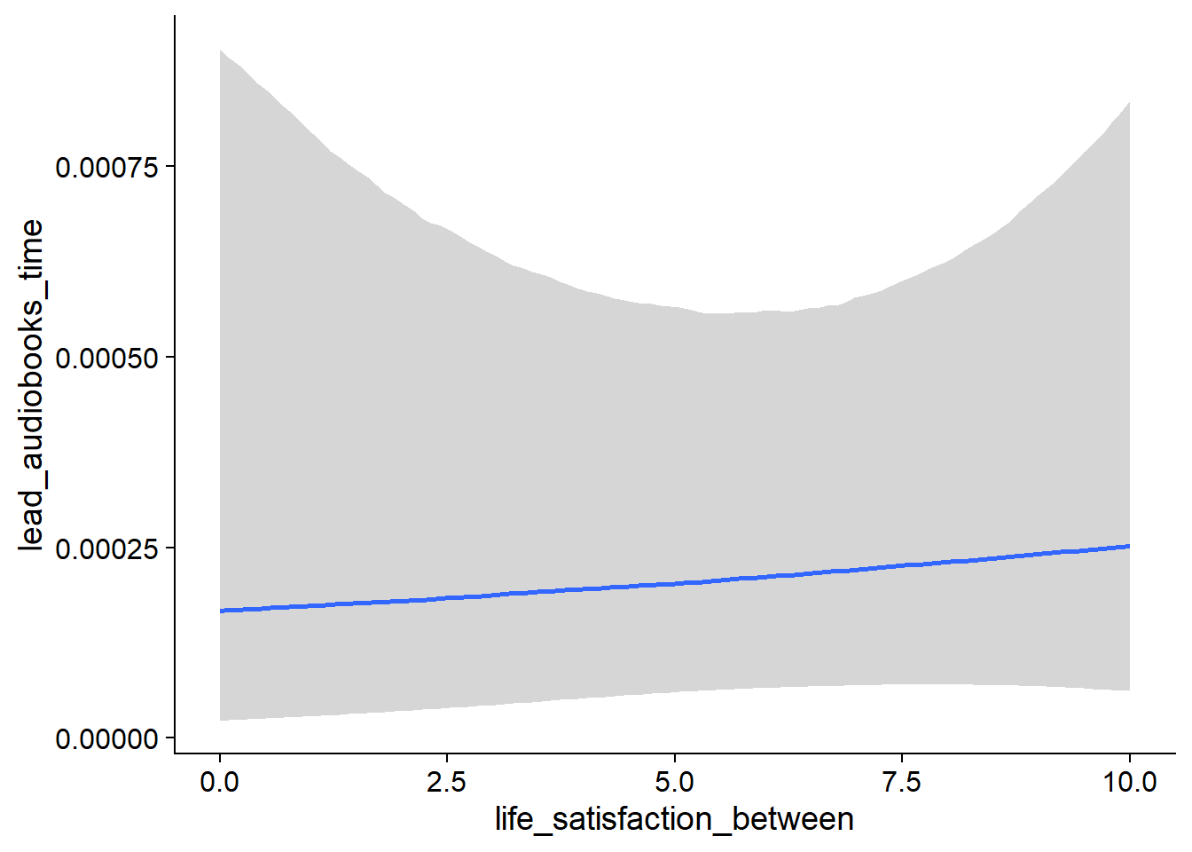
Figure 4.195: Conditional effects for Life Satisfaction-Audiobooks model
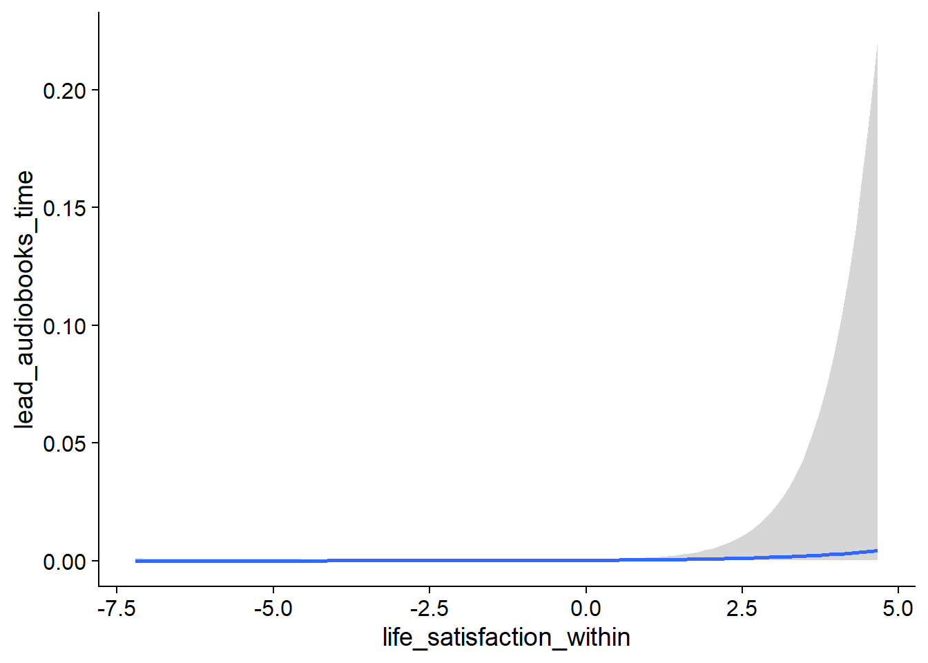
Figure 4.196: Conditional effects for Life Satisfaction-Audiobooks model
##            used  (Mb) gc trigger   (Mb)  max used   (Mb)
## Ncells  3694348 197.3    6044351  322.9   6044351  322.9
## Vcells 23791806 181.6  192291044 1467.1 255811179 1951.7