2 Data processing
Let’s process the raw data and get them to a format that we can work with for the analysis. The study has three raw data files:
personality_raw.csvis the survey participants filled out at the beginning of the study, reporting personality traitsdiary_raw.csvis the end of day survey participants filled out during the diary part of the studyscreen_time_raw.csvis the objective screen time data participants reported
2.1 Personality data
The data are on the OSF.
You can download them if you set the code chunk below to eval=TRUE.
Downloading only works when the OSF project is public.
If it isn’t during peer review, you’ll need to paste the data files from the OSF to the data/ folder manually.
# create directory
dir.create("data/", FALSE, TRUE)

# download models
osf_retrieve_node("https://osf.io/7byvt/") %>%
  osf_ls_nodes() %>%
  filter(name == "data") %>%
  osf_ls_files(
    .,
    n_max = Inf
  ) %>%
  osf_download(
    .,
    path = here("data"),
    progress = FALSE
  )
## # A tibble: 4 x 4
## name id local_path meta
## <chr> <chr> <chr> <list>
## 1 diary_raw.csv 603e5635441575030c586bc7 data/diary_raw.csv <named list [3]>
## 2 personality_raw.csv 603e5635035cf7031cc86382 data/personality_raw.csv <named list [3]>
## 3 processed_data.rds 603e56364415750312587b3a data/processed_data.rds <named list [3]>
## 4 screen_time_raw.csv 603e56374415750312587b48 data/screen_time_raw.csv <named list [3]>Let’s load the personality data.
personality_raw <- read_csv(here("data", "personality_raw.csv"))Qualtrics names aren’t very informative, so I give some sensible variable names (although this data set has mostly meaningful variable names).
Also, there are variables (i.e., anything starting with afi to selfreflect) that were part of a different study, which is why I don’t include them here.
Note that I don’t want to change the raw data object, so I’ll keep using personality as a new object from here on.
personality <-
  personality_raw %>%
  select(
    # meta data
    start_date = StartDate,
    end_date = EndDate,
    progress = Progress,
    duration = Duration__in_seconds_,
    finished = Finished,
    recorded_date = RecordedDate,
    id = study_id,
    date,

    # basic psychological need satisfaction trait
    bpns_ = starts_with("bpns"),

    # big five
    big_five_ = starts_with("bfi"),

    # demographics
    gender,
    gender_entry = gender_3_TEXT,
    age = Q42,
    ethnicity_american_indian = ethnicity_1,
    ethnicity_asian = ethnicity_2,
    ethnicity_island = ethnicity_3,
    ethnicity_black = ethnicity_4,
    ethnicity_white = ethnicity_5,
    ethnicity_hispanic = ethnicity_6,
    ethnicity_multi = ethnicity_7
  )
Next, I make sure those variables have the correct variable type.
I’ll also recode factor levels so that labels are readable.
Note that participants filled in their age from a dropdown menu to prevent typos.
The dropdown went from age 18 (1) to 30+ (13).
Nobody was older than thirty, so I’ll recode age as well.
personality <-
  personality %>%
  mutate(
    id = paste0("pp_", id), # add pp for participant just so later I don't mistake the id variable for a count
    across( # turn those two into factors
      c(finished, id, gender),
      as.factor
    ),
    finished = fct_recode(
      finished,
      "yes" = "1",
      "no" = "0"
    ),
    gender = fct_recode(
      gender,
      "male" = "1",
      "female" = "2",
      "other" = "3"
    ),
    age = age + 17
  )
I see that ethnicity was multiple choice although “multiracial” is an answer option. So I think it makes more sense to combine this all into one variable. That required quite a lot of code, but was still less problematic than transforming the ethnicity variables to long format. I took the following steps:
- check who reported multiple ethnicities
- those who did get an
NAon all other ethnicity variables - recoded the variables from numeric to containing the ethnicity factor level and coalesce
personality <-
  personality %>%
  mutate(
    multiple = rowSums(select(., starts_with("ethnicity")), na.rm = TRUE), # check who reported multiple ethnicities

    # those with multiple get NA for all other ethnicity variables
    across(
      c(ethnicity_american_indian:ethnicity_hispanic),
      ~ case_when(
        multiple > 1 ~ NA_real_,
        TRUE ~ .
      )
    ),

    # turn into character which makes recoding below easier
    across(
      c(ethnicity_american_indian:ethnicity_hispanic),
      as.character
    ),

    # recode the individual variables
    ethnicity_american_indian = if_else(ethnicity_american_indian == 1, "American Indian/Alaska Native", NA_character_),
    ethnicity_asian = if_else(ethnicity_asian == 1, "Asian", NA_character_),
    ethnicity_island = if_else(ethnicity_island == 1, "Native Hawaiian or Other Pacific Islander", NA_character_),
    ethnicity_black = if_else(ethnicity_black == 1, "Black or African American", NA_character_),
    ethnicity_white = if_else(ethnicity_white == 1, "White", NA_character_),
    ethnicity_hispanic = if_else(ethnicity_hispanic == 1, "Hispanic or Latino", NA_character_),
    ethnicity_multi = if_else(multiple > 1, "Multiracial", NA_character_),

    # coalesce them (coalesce doesn't work with .select helpers, so needed to type the variables out)
    ethnicity = as.factor(
      coalesce(
        ethnicity_american_indian,
        ethnicity_asian,
        ethnicity_island,
        ethnicity_black,
        ethnicity_white,
        ethnicity_hispanic,
        ethnicity_multi
      )
    )
  ) %>%
  select(start_date:age, ethnicity)
Then I remove those cases without an id (aka test runs) and those with an id but not other entries.
The latter are probably no-shows.
Note: In the earlier versions of this script, I excluded per data set, which made it hard for reporting exact exclusions in the final paper.
For example, at this point I don’t know whether someone I exclude here even participated in the diary part of the study.
Therefore, I save each exclusion criterion in a separate object and inspect how many people we actually need to exclude later in the data merging section.
# remove test run
personality <-
  personality %>%
  filter(id != "pp_NA")

personality_exclusions_1 <-
  personality %>%
  filter(is.na(start_date)) %>%
pull(id)| na_count_row | n |
|---|---|
| 0 | 1 |
| 1 | 246 |
| 2 | 29 |
| 3 | 5 |
| 4 | 2 |
| 7 | 1 |
| 9 | 2 |
| 25 | 1 |
| 49 | 4 |
| 74 | 1 |
| 81 | 10 |
I’ll exclude the latter.
# exclude those with > 15 missing values (which identifies empty rows)
personality_exclusions_2 <-
  personality %>%
  mutate(
    na_count_row = rowSums(is.na(.))
  ) %>%
  filter(na_count_row >70) %>%
  pull(id)
Alright, time to construct the means for the scales. But first, I check data quality by seeing whether there are instances of “straightlining” (i.e., choosing the same response option for all items of a scale). We also had attention checks in the survey.
Let’s have a look at those attention checks. For itembpns_25 participants had to choose 2 as a response and for item big_five_45 they had to choose 5.
When we check Table 2.2, we see that 5 participants didn’t pass both attention checks.
|
|
|
I’ll exclude those participants because I don’t think we can trust their data.
personality_exclusions_3 <-
  personality %>%
  filter(bpns_25 != 2 & big_five_45 != 5) %>%
  pull(id)
Next, I check for straightlining by inspecting the variance per daily survey on the BPNS and BF scales. Turns out that it’s not super straightforward to compute variance per row, found help here.
personality <-
  personality %>%
    rowwise() %>%
    mutate(
      bpns_sd = sd(
        c_across(starts_with("bpns")),
        na.rm = TRUE
      ),
      big_five_sd = sd(
        c_across(starts_with("big_five")),
        na.rm = TRUE
      )
    ) %>%
  unnest(cols = c())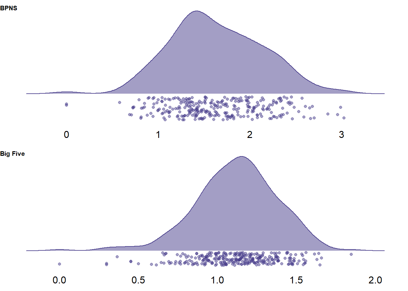
Figure 2.1: Distribution of variances per survey on two measures
Those two are already captured by the exclusion criteria above (I checked manually, but I’ll still save them in an object).
personality_exclusions_4 <-
  personality %>%
  filter(bpns_sd == 0 | big_five_sd == 0) %>%
  pull(id)
Alright, now we can aggregate the individual items to scale scores. Some of those items are reverse-coded (see the codebook for details). I’ll code all scales such that a higher scores means scoring more positively on that scale.
personality <-
  personality %>%
  mutate(
    across(
      c(
        bpns_5:bpns_8,
        bpns_13:bpns_15,
        bpns_21:bpns_25,
      ),
      function(.) 8 - .
    ),
    across(
      c(
        big_five_2,
        big_five_6,
        big_five_8,
        big_five_9,
        big_five_12,
        big_five_18,
        big_five_21,
        big_five_23,
        big_five_27,
        big_five_31,
        big_five_37,
        big_five_43
      ),
      function(.) 6 - .
    )
  )
Now I create the scales by taking the mean of the respective items. Note that I remove missing values in computing row means to ignore the occasional missing value. (For those with missing values throughout, see next code chunk.)
personality <-
  personality %>%
  mutate(

    # trait needs
    autonomy_trait = rowMeans(select(., bpns_1:bpns_8), na.rm = TRUE),
    competence_trait = rowMeans(select(., bpns_9:bpns_16), na.rm = TRUE),
    relatedness_trait = rowMeans(select(., bpns_17:bpns_24), na.rm = TRUE),

    # big five
    extraversion = rowMeans(
      select(
        .,
        big_five_1,
        big_five_6,
        big_five_11,
        big_five_16,
        big_five_21,
        big_five_26,
        big_five_31,
        big_five_36
      ),
      na.rm = TRUE
    ),
    agreeableness = rowMeans(
      select(
        .,
        big_five_2,
        big_five_7,
        big_five_12,
        big_five_17,
        big_five_22,
        big_five_27,
        big_five_32,
        big_five_37,
        big_five_42
      ),
      na.rm = TRUE
    ),
    conscientiousness = rowMeans(
      select(
        .,
        big_five_3,
        big_five_8,
        big_five_13,
        big_five_18,
        big_five_23,
        big_five_28,
        big_five_33,
        big_five_38,
        big_five_43
      ),
      na.rm = TRUE
    ),
    neuroticism = rowMeans(
      select(
        .,
        big_five_4,
        big_five_9,
        big_five_14,
        big_five_19,
        big_five_24,
        big_five_29,
        big_five_34,
        big_five_39
      ),
      na.rm = TRUE
    ),
    openness = rowMeans(
      select(
        .,
        big_five_5,
        big_five_10,
        big_five_15,
        big_five_20,
        big_five_25,
        big_five_30,
        big_five_35,
        big_five_40,
        big_five_41,
        big_five_44
      ),
      na.rm = TRUE
    )
  )
Last, some participants didn’t fill out the Big Five items, so they haven an NaN entry for those scales now.
I’ll turn that into an NA value
personality <-
  personality %>%
  mutate(
    across(
      c(autonomy_trait:openness),
      ~ na_if(.x, "NaN")
    )
  )
2.2 Diary data
Let’s load and inspect the diary data.
# load data
diary_raw <- read_csv(here("data", "diary_raw.csv"))
Qualtrics names aren’t very informative, so I give some sensible variable names.
Again, there are many variables (i.e., anything before Q21-1) that were part of a different study, which is why I don’t include them here.
Like before, I don’t want to change the raw data object, so I’ll keep using diary as a new object from here on.
diary <-
  diary_raw %>%
  select(
    # meta data
    start_date = StartDate,
    end_date = EndDate,
    progress = Progress,
    duration = Duration__in_seconds_,
    finished = Finished,
    recorded_date = RecordedDate,
    id = study_id,
    day = Day,
    date = Q27,

    # social media subjective estimates
    hours_subjective = Q21_1,
    minutes_subjective = Q21_2,
    pickups_subjective = Q22_1,
    notifications_subjective = Q23_1,

    # arousal
    low_positive_peaceful = Q24_1,
    low_positive_calm = Q24_2,
    low_positive_related = Q24_3,
    high_negative_anxious = Q24_4,
    high_negative_jittery = Q24_5,
    high_negative_tense = Q24_6,
    high_positive_happy = Q24_7,
    high_positive_energized = Q24_8,
    high_positive_excited = Q24_9,
    low_negative_sluggish = Q24_10,
    low_negative_sad = Q24_11,
    low_negative_gloomy = Q24_12,

    # autonomy need satisfaction
    autonomy_ = Q25_1:Q25_4,

    # competence need satisfaction
    competence_ = Q25_5:Q25_8,

    # relatedness need satisfaction
    relatedness_ = Q25_9:Q25_12,

    # experiences
    satisfied = Q30_1,
    boring = Q30_2,
    stressful = Q30_3,
    enjoyable = Q30_4
  )
Next, I make sure those variables have the correct variable type.
I’ll also recode factor levels so that labels are readable.
Note that day goes from 1 to 5.
All participants started on a Monday, which is why I turn day into a factor and reorder the levels.
diary <-
  diary %>%
  mutate(
    id = paste0("pp_", id), # add pp for participant just so later I don't mistake the id variable for a count
    across( # turn those two into factors
      c(finished, id, day),
      as.factor
    ),
    finished = fct_recode(
      finished,
      "yes" = "1",
      "no" = "0"
    ),
    day = fct_recode(
      day,
      "monday" = "1",
      "tuesday" = "2",
      "wednesday" = "3",
      "thursday" = "4",
      "friday" = "5"
    )
  )
Then I identify all empty rows (i.e., rows without a start date, so people who have placeholder id, but didn’t participate on that day).
diary_exclusions_1 <-
  diary %>%
  filter(is.na(start_date)) %>%
select(id, day)NAs there are per row in Table 2.3.
Most participants filled out everything, but a couple of them have basically empty rows (e.g., those with 30 or 40 missing values per row).
| na_count_row | n |
|---|---|
| 0 | 1072 |
| 1 | 49 |
| 2 | 16 |
| 3 | 3 |
| 4 | 1 |
| 6 | 1 |
| 8 | 1 |
| 9 | 2 |
| 16 | 1 |
| 20 | 1 |
| 23 | 1 |
| 28 | 2 |
| 32 | 24 |
| 39 | 336 |
I manually inspected those with more than 15 missing values and neither of them even finished any of the scales. Therefore, I’ll exclude them here.
# exclude those with > 15 missing values
diary_exclusions_2 <-
  diary %>%
  mutate(
    na_count_row = rowSums(is.na(.))
  ) %>%
  filter(na_count_row > 15) %>%
  mutate(id = droplevels(id)) %>%
  select(id, day)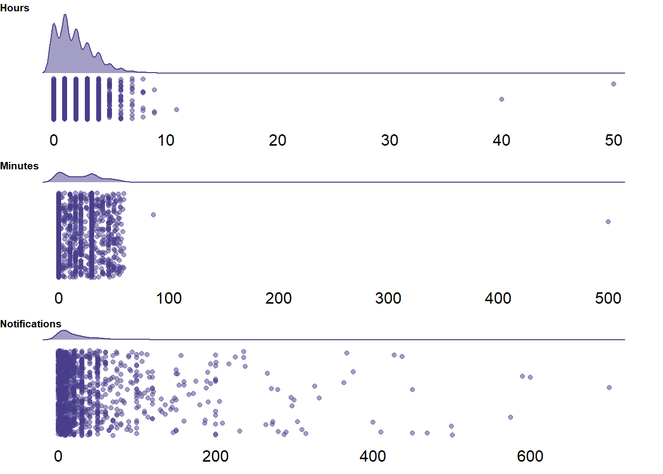
Figure 2.2: Distribution of self-reported social media indicators
For notifications, it’s hard to argue that it’s unrealistic that participants thought they got several hundred of them.
So I will leave those unchanged.
However, there are several outliers in hours_subjective and minutes_subjective.
I manually inspected those cases and it’s hard to tell whether participants just mixed up hours and minutes or whether their entry is indeed not meaningful.
One participant filled in 50h and 500min.
Another 40h.
For those two, I’ll set their subjective values to NA.
One participant filled in 5h and 86min.
The minutes entry might have been a typo, but it’s hard to tell what the participant meant, so I’ll set that to NA as well.
diary <-
  diary %>%
  mutate(
    hours_subjective = case_when(
      hours_subjective > 24 | minutes_subjective > 60  ~ NA_real_,
      TRUE ~ hours_subjective
    ),
    minutes_subjective = if_else(
      minutes_subjective > 60,
      NA_real_,
      minutes_subjective
    )
  )
Next, I check data quality further by seeing whether there are instances of “straightlining.” For that, I check the variance per daily survey on the well-being scale, need satisfaction, and experiences.
diary <-
  diary %>%
    rowwise() %>%
    mutate(
      well_being_sd = sd(
        c_across(low_positive_peaceful:low_negative_gloomy),
        na.rm = TRUE
      ),
      needs_sd = sd(
        c_across(autonomy_1:relatedness_4),
        na.rm = TRUE
      ),
      experiences_sd = sd(
        c_across(satisfied:enjoyable),
        na.rm = TRUE
      )
    ) %>%
  unnest(cols = c())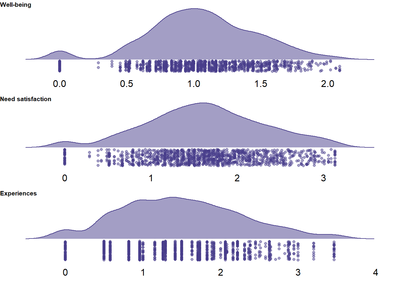
Figure 2.3: Distribution of variances per survey on three scales
In general, it’s not uncommon to select the same answer, especially for well-being measures. However, I’d be suspicious of those participants who straightlined for more than one scale (particularly the need satisfaction scale because it has quite a lot of items.) I’ll check how many surveys there are that have zero variance across those scales and how many participants there are who have at least one straightlining instance in more than 50% of their surveys.
diary <-
  diary %>%
  mutate(
    zero_variances = rowSums(
      select(., ends_with("_sd")) == 0, # count instances of zero variance across the three scales
      na.rm = TRUE
    )
)| zero_variances | n | percent |
|---|---|---|
| 0 | 1440 | 0.9536424 |
| 1 | 29 | 0.0192053 |
| 2 | 21 | 0.0139073 |
| 3 | 20 | 0.0132450 |
| id | total_surveys | total_straightline_surveys | percentage |
|---|---|---|---|
| pp_172 | 4 | 3 | 0.75 |
| pp_121 | 5 | 3 | 0.60 |
| pp_164 | 5 | 3 | 0.60 |
| pp_169 | 5 | 3 | 0.60 |
| pp_103 | 2 | 1 | 0.50 |
| pp_168 | 2 | 1 | 0.50 |
| pp_290 | 2 | 1 | 0.50 |
| pp_154 | 5 | 2 | 0.40 |
| pp_198 | 5 | 2 | 0.40 |
| pp_35 | 5 | 2 | 0.40 |
I will exclude those participants and then surveys with more than one instance of straightlining.
diary_exclusions_3 <-
c("pp_172", "pp_121", "pp_164", "pp_169", "pp_103", "pp_168", "pp_290")| zero_variances | n | percent |
|---|---|---|
| 0 | 1072 | 0.9571429 |
| 1 | 20 | 0.0178571 |
| 2 | 14 | 0.0125000 |
| 3 | 14 | 0.0125000 |
Alright, now we can aggregate the individual items to scale scores. Some of those items are reverse-coded. Namely, the third and fourth item for the need satisfaction subscales are reverse coded, as are all negative arousal items (if we want to create a score that shows higher well-being). See codebook for details.
# reverse code need items and arousal
diary <-
  diary %>%
  mutate(
    across(
      c(ends_with("_3"), ends_with("_4")),
      function(.) 8 - .
    ),
    across(
      contains("negative"),
      function(.) 6 - .
    )
  )
I create the scales by taking the mean of the respective items.
I also create a social_media_subjective measure by combining hours and minutes of estimated social media time.
diary <-
  diary %>%
  mutate(
    social_media_subjective = hours_subjective * 60 + minutes_subjective,
    well_being_state = rowMeans(select(., low_positive_peaceful:low_negative_gloomy), na.rm = TRUE),
    autonomy_state = rowMeans(select(., contains("autonomy")), na.rm = TRUE),
    competence_state = rowMeans(select(., contains("competence")), na.rm = TRUE),
    relatedness_state = rowMeans(select(., contains("relatedness")), na.rm = TRUE)
  )
Further, participants’ first day of participation was always a Monday. Specifically, three days in April 2019: the 15th, 22nd, 29th. Let’s check whether all of them indeed have their first day on one of those days.
Table 2.7 shows all day one surveys which were not recorded on one of those three dates. Indeed, everyone opened their first survey on one of the three start days. Some participants opened/recorded their answers right after midnight, which is fine.| id | start_date | recorded_date | duration | day |
|---|---|---|---|---|
| pp_21 | 2019-04-30 00:35:48 | 2019-04-30 00:57:14 | 1284 | monday |
| pp_61 | 2019-04-29 16:59:21 | 2019-05-06 17:00:41 | 72 | monday |
| pp_71 | 2019-04-22 16:01:29 | 2019-04-24 11:00:01 | 154711 | monday |
| pp_110 | 2019-04-22 20:16:35 | 2019-04-23 00:30:27 | 15231 | monday |
| pp_120 | 2019-04-23 00:08:15 | 2019-04-23 00:20:35 | 739 | monday |
| pp_192 | 2019-04-15 20:36:47 | 2019-04-16 00:27:47 | 13859 | monday |
| pp_201 | 2019-04-30 00:27:10 | 2019-04-30 00:52:59 | 1548 | monday |
| pp_211 | 2019-04-22 17:24:37 | 2019-04-23 12:13:59 | 67761 | monday |
| pp_257 | 2019-04-30 00:52:05 | 2019-04-30 01:21:55 | 1789 | monday |
| pp_265 | 2019-04-29 23:28:18 | 2019-04-30 01:34:43 | 7584 | monday |
| pp_275 | 2019-04-29 16:20:39 | 2019-05-06 16:31:47 | 648 | monday |
pp_71 took two days to respond to a survey.
| id | start_date | recorded_date | duration | day |
|---|---|---|---|---|
| pp_71 | 2019-04-22 16:01:29 | 2019-04-24 11:00:01 | 154711 | monday |
I guess it’s normal that participants open the survey late, forget it, and fill it out when they next day when they wake up. Because they’re students, waking up might be quite late, so I’ll check in Table 2.9 how many of them responded to a survey later than 10am the next day. Two participants were really late (i.e., responded after noon).
## Joining, by = c("id", "day")
## Joining, by = c("id", "day")| id | start_date | recorded_date | duration | day |
|---|---|---|---|---|
| pp_53 | 2019-04-18 16:11:51 | 2019-04-19 10:08:16 | 64584 | thursday |
| pp_71 | 2019-04-22 16:01:29 | 2019-04-24 11:00:01 | 154711 | monday |
| pp_98 | 2019-04-30 17:21:21 | 2019-05-01 12:03:12 | 67310 | tuesday |
| pp_161 | 2019-05-02 18:15:49 | 2019-05-03 10:05:25 | 56975 | thursday |
| pp_162 | 2019-04-30 22:00:37 | 2019-05-01 10:52:15 | 46297 | tuesday |
| pp_211 | 2019-04-22 17:24:37 | 2019-04-23 12:13:59 | 67761 | monday |
| pp_211 | 2019-04-23 23:40:53 | 2019-04-24 10:30:27 | 38972 | tuesday |
| pp_244 | 2019-04-19 18:45:44 | 2019-04-20 11:52:12 | 61587 | friday |
I manually checked the data from all those participants who filled out surveys so late that two surveys were recorded on the same day.
pp_71 responded to the Monday survey on Wednesday, in addition to the “regular” Wednesday survey.
For that reason, we can’t know whether day one refers to Monday or Tuesday.
All other participants are fine: They sometimes recorded their response late, but their response pattern shows no indication that they couldn’t refer to a clear day in their response.
Therefore, I remove the day one survey of pp_71 because we can’t tell to which day it refers, but leave the rest as is.
diary_exclusions_4 <-
  tibble(id = "pp_71", day = "monday")
2.3 Screen time data
Load the screen time data.
screen_time_raw <- read_csv(here("data", "screen_time_raw.csv"))Alright, the data are extremely wide because of the Qualtrics format. There are 220 variables in total. The data look like this:
- Total time over the past week of social media, plus total time per day (
Q2_1toQ10_2) - Typing in the top ten social networking media (
Q4_1toQ4_10) - Then participants filled in 13 items for each of those ten apps, first total time and notifications for the week for that app, then hours and minutes per day for that app (total 130 items,
Q3_1toQ76_2) - Then participants reported six items per each of the ten apps, the first of which was overall pickups in the past week, followed by pickups for each day of the week (
Q17_1_TEXTtoQ17_10_5)
Before turning the data into long format, I need to give some sensible variables names. However, manually renaming all variables is a real pain. So I’ll create the names systematically and store them in a vector, then assign them to the variables.
# define days
days <-
  c(
    "monday",
    "tuesday",
    "wednesday",
    "thursday",
    "friday"
  )

# the list of apps
apps <-
  paste0(
    rep("app_", 10),
    1:10
  )

# add hours and minutes to apps
apps_times <-
  paste0(
    rep(apps, each = 6*2),
    "_",
    c("hours", "minutes")
  )

# the overall time per week and day
names1 <-
  paste0(
    rep(c("hours_total_", "minutes_total_"),6),
    rep(c("week", days), each = 2)
  )

# now app, minutes, hours, per day
names2 <-
  paste0(
    apps_times,
    "_",
    rep(c("week", days), each = 2)
  )

# notifications per day
names3 <-
  paste0(
    apps,
    "_",
    "notifications",
    "_week"
  )

# pickups per week and day
names4 <-
  paste0(
    rep(apps, each = 6),
    "_pickups_",
    rep(c("week", days), 6)
  )
Then I apply those names. Once more, I use a new object and don’t overwrite the raw data.
# let's rename
screen_time <-
  screen_time_raw %>%

  # meta-data
  rename(
    start_date = StartDate,
    end_date = EndDate,
    progress = Progress,
    duration = Duration__in_seconds_,
    finished = Finished,
    recorded_date = RecordedDate,
    id = study_id
  ) %>%

  # the overall time per week and day
  rename_with(
    ~ names1,
    Q2_1:Q10_2
  ) %>%

  # the top ten apps
  rename(
    app_ = Q4_1:Q4_10
  ) %>%

  # now rename all app minutes and hours per day
  rename_with(
    ~ names2,
    c( # except the notifications because they don't fit the pattern
      Q3_1:Q76_2,
      -Q11_1,
      -Q22_1,
      -Q78_1,
      -Q29_1,
      -Q43_1,
      -Q36_1,
      -Q50_1,
      -Q57_1,
      -Q64_1,
      -Q71_1
    )
  ) %>%

  # the past week notifications per app
  rename_with(
    ~ names3,
    c(
      Q11_1,
      Q22_1,
      Q78_1,
      Q29_1,
      Q43_1,
      Q36_1,
      Q50_1,
      Q57_1,
      Q64_1,
      Q71_1
    )
  ) %>%

  # rename pickup variables
  rename_with(
    ~ names4,
    Q17_1_TEXT:Q17_10_5
  ) %>%

  # only keep variables of interest
  select(
    -Status
  )

# remove name objects (they were only temp files)
rm(apps, apps_times, days, names1, names2, names3, names4)
Before I assign variables types and factor levels, I saw that, for some reason, the past week’s number of pickups for each app have text entries, not numerical (i.e., "twenty one" instead of 21).
I know that the english package can translate numbers to words, but not the other way around.
Thank god, someone has written a function for this, see full details here.
The function is in the Setting up chapter.
Note that this word2num function doesn’t work well with the word “and.”
For example, "three hundred and eleven" turns into 611, but "three hundred eleven" turns into the correct 311.
Therefore, I first remove all “and”s from those variables, then apply the function.
Similarly, I’ll replace all “a” with “one” (e.g., “a hundred” to “one hundred”).
One participant also replied with a string (that they access facebook via their browser), so I’ll set that to NA.
screen_time <-
  screen_time %>%
  mutate(
    across(
      ends_with("pickups_week"),
      ~ case_when(
        .x == "NA because accessed Facebook through Safari" ~ NA_character_,
        .x == "NA because accessed Twitter through Safari" ~ NA_character_,
        TRUE ~ .x
      )
    ),
    across(
      ends_with("pickups_week"),
      ~ str_remove(.x, "and")
    ),
    across(
      ends_with("pickups_week"),
      ~ str_replace(.x, "A ", "one ")
    )
  ) %>%
  rowwise() %>%
  mutate(
    across(
      ends_with("pickups_week"),
      word2num
    ),
    across(
      ends_with("pickups_week"),
      unlist
    )
  ) %>%
  unnest(cols = c())
Next, I assign correct variable types and factor levels.
screen_time <-
  screen_time %>%
  mutate(
    id = paste0("pp_", id),
    across( # turn those two into factors
      c(finished, id),
      as.factor
    ),
    finished = fct_recode(
      finished,
      "yes" = "1",
      "no" = "0"
    )
  )
Then I exclude empty rows.
The data set has all participant numbers even when they didn’t participate, so I’ll identify those without a start date as well as those who didn’t fill in app_1, which means they have empty rows other than the meta-data.
screen_time_exclusions_1 <-
  screen_time %>%
  filter(is.na(start_date) | is.na(app_1)) %>%
  mutate(id = droplevels(id)) %>%
  pull(id)
At this point, the data set has measures on two levels: per app and time frame (day, full week), and the total times across all apps per day.
I think it’s easiest to separate the data.
The per app data are only informative for plotting and descriptives, but the actual data we’re interested in are the total times summed across all apps.
So I’ll first get the per data app (excluding empty rows temporarily from screen_time).
Note that I add the names of the apps in a separate step and then calculate the objective social media time.
# turn app data long
apps_long <-
  screen_time %>%
    filter(!is.na(start_date)) %>%
    filter(!is.na(app_1)) %>%
    mutate(id = droplevels(id)) %>%
  select(
    start_date:id,
    app_1_hours_week:app_10_pickups_friday
  ) %>%
  pivot_longer(
    cols = c(app_1_hours_week:app_10_pickups_friday),
    names_to = c(
      "app",
      "rank",
      "measure",
      "time_frame"
    ),
    names_sep = "_"
  ) %>%
  pivot_wider( # then spread the measure variable which now contains hours, minutes, notifications, pickups
    names_from = "measure",
    values_from = "value"
  ) %>%
  select(-app) # redundant

# get the names of the apps
app_names <-
  screen_time %>%
  filter(!is.na(start_date)) %>%
  filter(!is.na(app_1)) %>%
  mutate(id = droplevels(id)) %>%
  select(
    id,
    app_1:app_10
  ) %>%
  pivot_longer(
    -id,
    names_to = c("app", "rank"),
    names_sep = "_"
  ) %>%
  select(-app) %>% # redundant
  rename(
    app = value # contains name of app
  )

# add them to the long data set
apps_long <-
  left_join(
    apps_long,
    app_names,
    by = c("id", "rank")
  ) %>%
  relocate(
    app,
    .after = rank
  ) %>%

  # if someone only filled in minutes, but not hours, turn hours to 0
  mutate(
   hours = case_when(
    is.na(hours) & is.na(minutes) ~ NA_real_,
    is.na(hours) & !is.na(minutes) ~ 0,
    TRUE ~ hours
   ),

   # when someone only filled in hours, but not minutes, turn minutes to 0
   minutes = case_when(
     is.na(hours) & is.na(minutes) ~ NA_real_,
     !is.na(hours) & is.na(minutes) ~ 0,
     TRUE ~ minutes
   ),

   # total time
   social_media_objective = hours * 60 + minutes
  )
Then I get the total times across all apps in the long format. Note that participants reported their screen time on the weekend. Thus, their reports for week will not be identical with the sum of Monday to Friday, because the screen time feature measures time on the weekend as well (aka additional screen time measured from the end of Friday until the moment they reported their weekly screen time).
# get total screen time (of all social media apps in long format)
totals_long <-
  screen_time %>%
  filter(!is.na(start_date)) %>%
  filter(!is.na(app_1)) %>%
  mutate(id = droplevels(id)) %>%
  select(
    id,
    hours_total_week:minutes_total_friday
  ) %>%
  pivot_longer(
    -id,
    names_to = c(
      "measure",
      "total",
      "time_frame"
    ),
    names_sep = "_"
  ) %>%
  select(-total) %>% # redundant

  pivot_wider( # spread hours and minutes
    names_from = "measure",
    values_from = "value"
  ) %>%

  # same as above: if one of the two measures (hours or minutes) has an entry and the other is NA, we set that NA to 0
  mutate(
    hours = case_when(
      is.na(hours) & is.na(minutes) ~ NA_real_,
      is.na(hours) & !is.na(minutes) ~ 0,
      TRUE ~ hours
    ),

  # when someone only filled in hours, but not minutes, turn minutes to 0
    minutes = case_when(
      is.na(hours) & is.na(minutes) ~ NA_real_,
      !is.na(hours) & is.na(minutes) ~ 0,
      TRUE ~ minutes
    ),

   # total time
    social_media_objective = hours * 60 + minutes
  )
The totals_long is the data set of interest because it has total screen time per day, which we can match with the diary data.
Thus, to arrive at the final sample size, we’ll only keep participants who have data in the diary data set.
For merging, we’ll need to exclude those participants in totals_long who don’t have a match in diary.
But first, I check how much the sum of total time across apps per day in total_long converges with the sum of time across all apps per day in apps_long.
There will definitely be differences, simply because participants have more chances to make typos when reporting the individual apps per day (in apps_long) compared to reporting the overall time across all apps once per day (in total_long).
Also, participants will occasionally skip an individual app per day rating.
Below, I get the total time per day across all ten apps and then join that estimate with the data set containing the total times (total_long).
Afterwards, per day, I see how much the two variables differ.
# get total time across apps per day
apps_aggregated <-
  apps_long %>%
  group_by(id, time_frame) %>%
  filter(time_frame != "week") %>% # no week
  summarise(total_time = sum(social_media_objective, na.rm = TRUE))

# join with total times
compare <-
  left_join(
    totals_long %>%
      filter(time_frame != "week"),
    apps_aggregated
  ) %>%

  # and compute a deviance score
  mutate(
    difference = social_media_objective - total_time
  )
Overall, the two sums of use across apps and days are highly similar, with a mean difference of M = 4.09, SD = 17.4 and an extremely high correlation, r = 0.98.
There were some missing values in the total social media time per day that participants reported. I check who has missing data on any of the weekdays in thetotals_long data set.
We can check whether those participants have reported individual app use for that day and use an aggregate over apps on that day as a substitute, given their high correlation.
In other words: When participants forgot to report their overall social media use for a day, but reported use for all social media apps they used on that day, we can just use the sum of those social media apps as a replacement for overall social media use.
However, we see in 2.10 that all participants reported social media screen time across all days, so no need for imputation.
| id | time_frame | hours | minutes | social_media_objective | total_time | difference |
|---|---|---|---|---|---|---|
| 0 | 0 | 0 | 0 | 0 | 0 | 0 |
Before I merge all data sets, I need to add the objective notifications and pickups (currently in apps_long) to the totals_long data set.
Note that at the time of the study, iOS screen time wouldn’t report notifications for app per day, only for the past week.
Therefore, the weekly notifications have the same caveat as the weekly screen time: they will include a couple of notifications that participants received on the day they retrospectively reported their objective use.
For pickups, as with screen time, we can sum up all days to get an accurate measure of week’s pickups.
I’ll sum up both pickups and notifications over participant.
Pickups will be per day, but notifications only per week.
I then add pickups to the totals_long data set.
Notifications I’ll add later during merging (because they are not aggregated per day).
# get total pickups across apps per day
pickups_aggregated <-
  apps_long %>%
  group_by(id, time_frame) %>%
  filter(time_frame != "week") %>% # no week
  filter(!is.na(pickups)) %>% # exclude missing values (if I do na.rm = T in sum below it will result in zeros to sum NAs)
  summarise(pickups_objective = sum(pickups))

# get notifications across apps per participant
notifications_aggregated <-
  apps_long %>%
  group_by(id) %>%
  summarise(weekly_notifications = sum(notifications, na.rm = TRUE))

# add pickups to totals_long
totals_long <-
  left_join(
    totals_long,
    pickups_aggregated,
    by = c("id", "time_frame")
  )
2.4 Merge data sets
Finally, we can merge the three data sets. Before I do any merging, I’ll check out the number of data points per data set and the ones they have in common before I count exclusions. This is mostly for reporting in the paper.
# number of participants who took initial survey (take out empty rows)
personality %>%
  filter(!id %in% personality_exclusions_1) %>%
  pull(id) -> personality_n

length(personality_n)
## [1] 292# number of those who also participated in diary part
diary %>%
anti_join(., diary_exclusions_1) -> diary_n## Joining, by = c("id", "day")length(unique(diary_n$id))## [1] 275# number of those who came back to report screen time
screen_time %>%
filter(!id %in% screen_time_exclusions_1) %>%
pull(id) -> screen_time_n
length(screen_time_n) ## [1] 97The diary data set is the “base” because it has our variables of interest and the correct time structure.
To that data set we add the objective social media measures from the totals_long data set.
The identifier for a survey are the participant id and the day on which they filled out a survey/for which they reported objective use.
Note that we omit the meta-data from totals_long (e.g., start_date) because they are different from the meta-data of diary.
We also only keep the variables of interest from here on, meaning I’ll exclude some variables that aren’t informative.
dat <-
  left_join(

    # the diary data with only relevant variables
    diary %>%
      select(
        duration_diary = duration, # so that we can get filling out times for each data set
        id:day,
        pickups_subjective:enjoyable, # don't need individual minutes and hours anymore
        social_media_subjective:relatedness_state
      ),

    # the objective totals with only relevant variables
    totals_long %>%
      filter(time_frame != "week") %>%
      rename(
        day = time_frame
      ) %>%
      select(id, day, social_media_objective, pickups_objective),

    # joining by the two identifiers
    by = c("id", "day")
  )
The merging above kept all cases of diary and added variables from totals_long when there was a match, otherwise setting the new variables to NA.
Therefore, I remove all cases which have NA on the added variables to get to our final sample.
(There were no missings in the social_media_objective variable.)
In other words, this removes those participants who didn’t fill out the screen time survey.
dat <-
  dat %>%
  filter(!is.na(social_media_objective))
For descriptive information, I’ll also add the survey duration of the screen time data.
dat <-
  left_join(
    dat,
    screen_time %>%
      select(id, duration) %>%
      rename(
        duration_screen_time = duration
      ),
    by = "id"
  )
Okay, then I add the personality variables.
Again, dat is the “master” and we add personality variables (aka traits from personality), omitting variables that aren’t of interest.
dat <-
  left_join(
    dat,
    personality %>%
      select(
        duration_personality = duration,
        id,
        bpns_1:openness
      ),
    by = "id"
  )
Then, I add the notifications over one week as a constant.
dat <-
  left_join(
    dat,
    notifications_aggregated,
    by = "id"
  )
Alright, only keeping those who had screen time measures already removed a large number of cases, some of them were part of the exclusions for both the personality and the diary parts.
I now apply all exclusions (if necessary) to get to the final data set.
Note that I don’t exclude those in diary_exclusions_2 after all: Those are the ones who didn’t fill in an experience sampling survey, but all of them still have personality scores and the retrospective screen time estimates.
## personality

# nobody left who didn't fill in the personality survey
unique(dat$id %in% personality_exclusions_1)
## [1] FALSE# and nobody with empty rows
unique(dat$id %in% personality_exclusions_2)## [1] FALSE# the people who failed attention checks either didn't fill out the diary or the screen time part
unique(dat$id %in% personality_exclusions_3)## [1] FALSE# same goes for personality straightliners
unique(dat$id %in% personality_exclusions_4)## [1] FALSE## diary
# some people with empty diary entries left, nobody left who didn't participate in the diary (no wonder, we used diary as the base for merging)
# those people will have empty diary entries, but still data for screen time, so no need to exclude them here, they'll be dropped from analysis automatically because of NA
inner_join(diary_exclusions_1, dat %>% select(id, day)) %>% nrow()## Joining, by = c("id", "day")## [1] 33# don't exclude anyone who missed a diary entry
# diary straightliners: need to exclude one person
dat$id[dat$id %in% diary_exclusions_3]## [1] pp_169 pp_169 pp_169 pp_169 pp_169
## 303 Levels: pp_1 pp_10 pp_100 pp_101 pp_102 pp_103 pp_104 pp_105 pp_106 pp_107 pp_108 pp_109 pp_11 pp_110 pp_111 ... pp_NAdat <-
dat %>%
filter(!id %in% diary_exclusions_3)
# last, exclude one diary entry that was provided too late (see details above)
dat <-
dat %>%
anti_join(., diary_exclusions_4)## Joining, by = c("id", "day")## screen time exclusions
# those with empty rows will have been excluded as we merged diary with totals_long (totals long excluded those who had all NA)
unique(dat$id %in% screen_time_exclusions_1)## [1] FALSEGood, then we have our final data set.
Because screen time was filled in retrospectively in the third session, those who didn’t fill in an experience sample will have NAs on the self-reports, but still a row with data because screen time for that day is there.
So each person has five rows, except for that one participant who filled in one of the surveys too late.
Next, I create an accuracy score for the comparison of objective and subjective phone use indicators. The objective measure is our “true” estimate. We want to know how far off participants were, relative to that true value, in their estimate. For that, we calculate the percentage error by subtracting the objective value from the subjective value (to get difference) and dividing by the objective value (to get error percent). Afterwards, we multiply by 100 to get a percentage. Say I estimated 110 subjective minutes, but the true value (i.e., the objective minutes) is 100. Then the error is 10%, an overestimate. If I estimated 100 subjective minutes, but the true value is 110, the error is ~9%, an underestimate.
In my opinion, that is more intuitive than a difference score.
It’s easier to understand the magnitude of an error in percent (say 80%) than raw units (say 10 minutes).
However, percent error brings one complication with it: If participants estimated 0 social media use, percent error becomes meaningless.
0 - objective / objective will always lead -100%.
There’s 11 cases with an estimate of zero, but actual, objective use.
It’s impossible in this case to determine an error percentage, simply because 0 is meaningless in the formula.
I could use a difference score instead, but that’ll make the interpretation less intuitive.
Those zeros might’ve also been typos, given how rare zeros are in the sample.
I could set those error instances to missing, but in the analysis, we want to be able to compare coefficient predicting both social media and error.
Therefore, I’ll set all three variables to NA.
dat <-
  dat %>%
  mutate(
    # error social media time
    error = (social_media_subjective - social_media_objective) / social_media_objective * 100,
    across(
      c(social_media_subjective, social_media_objective, error),
      ~ if_else(error == -100, NA_real_, .x)
    )
  )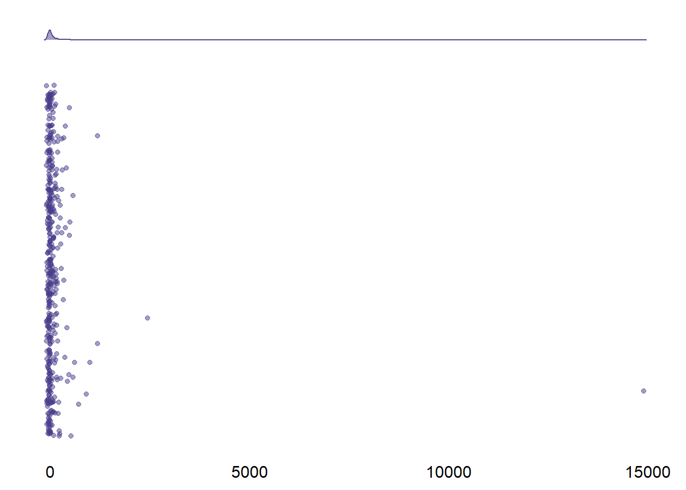
Figure 2.4: Distribution of percent error for screen time
I checked their raw data: One participant indicated exactly five hours, but probably meant five minutes (i.e., the participant with an error of 1.49^{4}.
Similarly, the second largest entry seems to be a typo (i.e., 58 minutes).
I’ll set those all entries that are larger than 1500% to NA.
Also, one participant had zero objective time and zero subjective time.
Dividing by zero to get error above leads to NaN, so I’ll set that NA.
dat <-
  dat %>%
  mutate(
    error = if_else(error > 1500, NA_real_, error),
    error = if_else(
      social_media_subjective == 0 & social_media_objective == 0, NA_real_, error
    )
  )
Last, some housekeeping, reordering variables and making sure they all have the correct variable type, plus reordering the day factor.
dat <-
  dat %>%
  select(
    id,
    age:ethnicity,
    gender,
    starts_with("duration"),
    day,
    social_media_subjective,
    pickups_subjective,
    notifications_subjective,
    social_media_objective,
    error,
    pickups_objective,
    weekly_notifications,
    well_being_state:relatedness_state,
    low_positive_peaceful:enjoyable,
    autonomy_trait:openness,
    bpns_1:big_five_45
  ) %>%
  mutate(
    id = droplevels(id),
    day = as.factor(day),
    day = fct_relevel(
      day,
      "monday",
      "tuesday",
      "wednesday",
      "thursday",
      "friday"
    )
  )
When plotting the app data I want them to reflect the final sample, which is why I only keep those participants and surveys in the apps_long data set that are also in the final data set (i.e., dat).
I can’t just exclude those participants in apps_long because I also excluded surveys in diary on which dat is based.
Therefore, I only keep those entries in apps_long which have a corresponding row in dat (aka entries in both id and day).
Also, I’ll remove “week” as a time frame and add the notifications for that app over whole week as a constant per app.
apps_week <-
  apps_long %>%
  select(
    id,
    time_frame,
    app,
    rank,
    notifications
  ) %>%
  filter(time_frame == "week") %>%
  select(-time_frame)

apps_long <-
  left_join(

    # only those participants and days that are in final data set
    dat %>%
      select(id, day),

    # and the rest of the variables from apps_long, but without week
    apps_long %>%
      rename(day = time_frame) %>%
      filter(day != "week") %>%
      select(-notifications),

    by = c("id", "day")
  ) %>%

  # add the notifications for that app per week as a constant
  left_join(
    .,
    apps_week,
    by = c("id", "app", "rank")
  ) %>%
  select(id, day, rank:notifications) %>%
  rename(notifications_per_week = notifications)
Last, there are some NaNs in the data set after the transformations.
I’ll turn them into missings (i.e., NA).
dat <-
  dat %>%
  mutate(
    across(
      everything(),
      ~ na_if(.x, "NaN")
    )
  )
Write the analysis file.
write_rds(dat, here("data", "processed_data.rds"))