4 Analysis

I move on to the analyses. We have about a dozen models to run. All of these models should take into account that the data are nested (in participants and days). That means quite complex model structures, especially when we have many predictors. The lme4 package can handle such multi-level models, but in my experience suffers from many convergence issues that a Bayesian approach (i.e., the brms package) can handle better (see this paper for a comparison on convergence). Moreover, corrections for multiple comparisons are less of a problem with Bayesian models. Last, although the models here are mostly exploratory, we can still incorporate prior knowledge from the literature (and common sense about our variables).

4.1 Research questions

We have a total of 9 research questions. I divide them in three blocks:

To what extent do specific person-level variables such as personality and motivational factors shape the accuracy of social media time engagement?
To what extent do subjective experiences such as mood predict and or interact with person-level factors to shape the accuracy of social media time engagement?
What are the unique relations relating objective and subjective engagement to well-being outcomes?

Each of those questions comes with a number of models. I’ll structure the analysis section according to those blocks.

4.2 Data preparation

I processed the dat data set in previous sections. Specifying priors on the untransformed variables can be tough. In some analyses (e.g., predicting social media use) I’ll use centered predictors to make it easier to interpret the intercept. In other analyses (e.g., predicting error), I want to standardize outcomes and predictors of interest because standardized variables make it easier to choose sensible priors, especially because we can use standardized effect sizes reported in the literature. Standardizing also makes it easier to interpret the effect sizes.

First, I transform all variables of interest (into new variables).

dat <- 
  dat %>% 
  # center personality variables
  mutate(
    across(
      c(
        autonomy_state:relatedness_state,
        satisfied:enjoyable,
        autonomy_trait:openness
      ),
      ~ scale(.x, center = TRUE, scale = FALSE),
      .names = "{col}_c" # add "_c" suffix to new variables for "centered"
    )
  )

Next, let’s have a look of how many NAs there are per variable. Table 4.1 shows that missing values aren’t a big problem. The missings come from rows where participants didn’t answer the diary, but did report screen time mostly.

Table 4.1: Missing values per variable (column)
name	value
social_media_subjective	51
pickups_subjective	38
notifications_subjective	38
social_media_objective	51
error	53
pickups_objective	30
weekly_notifications	0
well_being_state	40
autonomy_state	39
competence_state	39
relatedness_state	39
satisfied	42
boring	42
stressful	41
enjoyable	44
autonomy_trait	0
competence_trait	0
relatedness_trait	0
extraversion	0
agreeableness	0
conscientiousness	0
neuroticism	0
openness	0

4.3 Do trait variables predict social media use and accuracy?

Our first research question asks whether personality traits and trait motivations predict the accuracy of social media time engagement. Specifically, we have three models that address the following sub-questions:

Do person-level variables predict objective-only engagement?
Do person-level variables predict subjective-only engagement?
Do person-level variables predict accuracy?

I’ll construct a model for each of those three questions. Our dependent variables are clear-cut: social_media_objective, social_media_subjective, and error.

Our predictors will be variables on the person-level, so trait/personality variables: the Big Five and the three self-determination motivations.

Note, I saved all brms model objects and load them below. Each model takes quite some time and the files get large (a total of half a GB). If you’re reproducing the analysis and don’t want to run the models yourself, you can download the model objects from the OSF. For that, you need to set the code chunk below to eval=TRUE, which creates a model/ directory with all models inside.

# create directory
dir.create("models/", FALSE, TRUE)

# download models
osf_retrieve_node("https://osf.io/7byvt/") %>% 
  osf_ls_nodes() %>% 
  filter(name == "models") %>% 
  osf_ls_files(
    .,
    n_max = Inf
  ) %>% 
  osf_download(
    .,
    path = here("models"),
    progress = FALSE
  )

4.3.1 Model 1: Trait variables predicting objective use

First, I choose sensible priors. There’s some literature out there on Big Five and smartphone use, as well as motivations and smartphone use. If we only knew the mean and variance of the social media estimates, a Gaussian distribution would be most appropriate. However, we do know more than just those two parameters. Namely, we know that the scale is continuous (i.e., time) and cannot be less than zero. Also, if we look at the distribution of time on an activity, the variance usually increases with the mean. Therefore, a gamma distribution appears more adequate to me.

That means the models will use a log-link, which makes it hard to have an intuition about prior distributions (at least for me). Thus, I follow the recommendations of McElreath and simulate the priors.

For the intercept, we can look at previous research. For example, this paper has average phone use times of about two hours per participant per day. Here, we only looked at social media use, so as a guess-timate with reasonable uncertainty, I’ll choose a lognormal distribution with a meanlog of 4.5 and a meansd of 0.8. See the upper left panel of Figure 4.1. That intercept has mots its value below two hours, but allows substantial skew for a couple of heavy users.
For the shape of the gamma distribution, I also played around and settled on one that somewhat resembles our assumptions on the intercept, such that the majority of values will be below five hours with a couple of heavy users (see left side upper panel).
For the Big Five fixed effects, this paper predicted social media use with the Big Five over two time period in a longitudinal design. They found that only neuroticism was related to social media use, but that effect was extremely small (\(\beta\) = .028). None of the other effects were large. Therefore, I’ll use rather flat, weakly regularizing priors for those effects. In 4.1, lower panel, I’ll use the prior on the left, because it’s skeptical, but regularizing. The one on the right might be too optimistic by suggesting a small positive effect.
For basic psychological needs, there’s quite some literature on these needs and pathological smartphone use (“smartphone addiction”). However, there’s little info we could use for priors, so I’ll just go with the same prior as for the Big Five. See the top right of the Figure below.
For all other parameters, I’ll take the brms default priors.

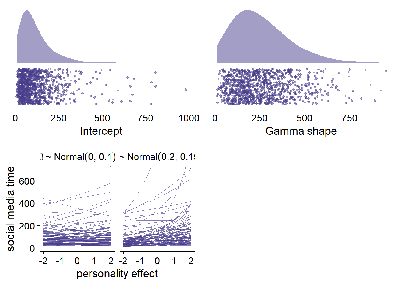
Credit for the code for the figures goes to Solomon Kurz.

Figure 4.1: Prior simmulations for Model 1

Let’s set those priors we simulated above.

priors_model1 <- 
  c(
    # intercept
    prior(normal(4.5, 0.8), class = Intercept),
    
    # prior on effects
    prior(normal(0, 0.1), class = b),
    
    # all other effects
    prior(gamma(2.5, 100), class = shape)
  )

Alright, time to run the model. Luckily, none of these variables have missing values, so I won’t need to model missings in this model. Note that I ran the block below once and stored the model. Those fit objects are too large for Github, so you can download them from the OSF. See the instructions in the Readme of the project.

model1 <- 
  brm(
    data = dat,
    family = Gamma(link = "log"),
    prior = priors_model1,
    social_media_objective ~
      1 +
      openness_c +
      conscientiousness_c +
      extraversion_c +
      agreeableness_c +
      neuroticism_c +
      competence_trait_c +
      relatedness_trait_c +
      autonomy_trait_c +
      (1 | id) +
      (1 | day),
    iter = 5000,
    warmup = 2000,
    chains = 4,
    cores = 4,
    seed = 42,
    control = list(adapt_delta = 0.99),
    file = here("models", "model1")
  )

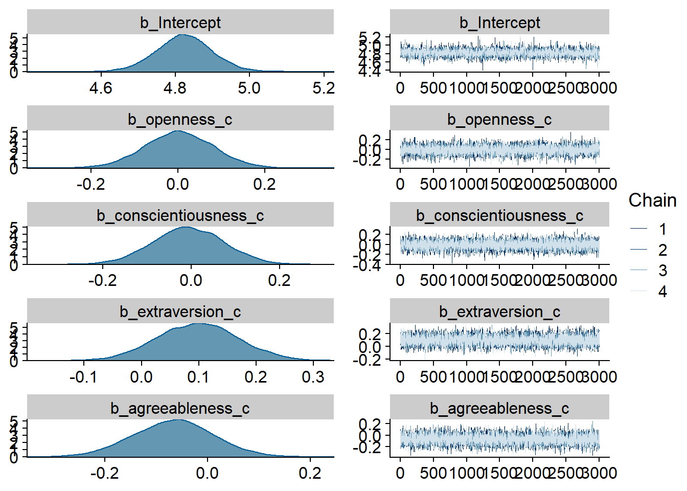
Let’s inspect the traceplots. Overall, they look fine and the chains seem to have mixed well, see (Figure ??). The residual standard deviation around the day grouping doesn’t look ideal though. Variation between days wasn’t that great, so the model estimates quite a lot variances that are close to zero. We could remove the day grouping, but I think we have theoretical reasons to keep it, namely to account for all known sources of variation.

Figure 4.2: Traceplots and posterior distributions for Model 1

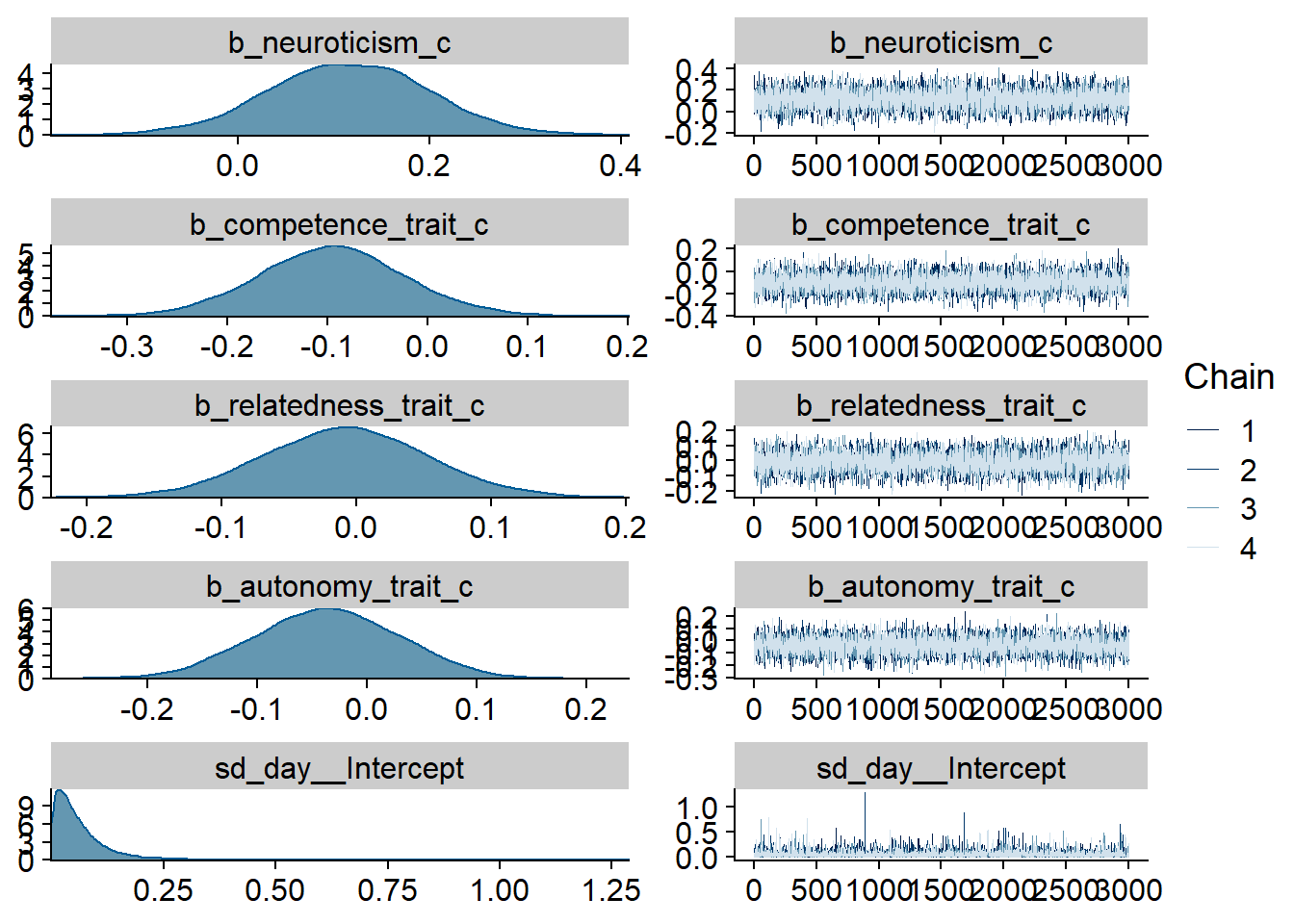
Figure 4.3: Traceplots and posterior distributions for Model 1

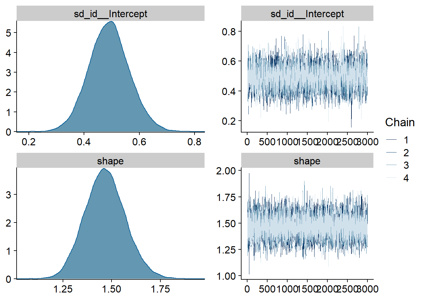
Figure 4.4: Traceplots and posterior distributions for Model 1

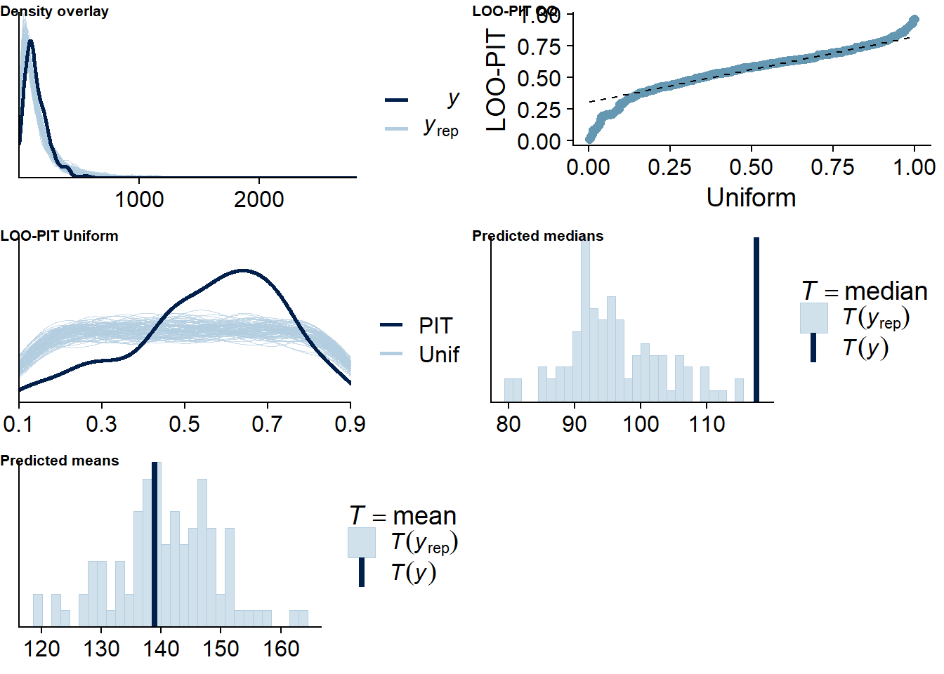
The posterior predictive distribution (Figure 4.5) shows that the model does an okay job in predicting our outcome, with little indication of overfitting. If anything, it looks like the model somewhat underestimates the social media time of users. Then again, the LOO-PIT graphs show that the model could be better, possibly because it doesn’t do the best job in predicting the majority of cases (i.e., the underestimate).

Figure 4.5: Posterior predictive checks for Model 1

Let’s also check for potentially influential values. None are tagged as influential, which increases my trust in the model.

loo(model1)

## 
## Computed from 12000 by 428 log-likelihood matrix
## 
##          Estimate   SE
## elpd_loo  -2440.0 14.4
## p_loo        20.7  1.4
## looic      4880.0 28.8
## ------
## Monte Carlo SE of elpd_loo is 0.1.
## 
## All Pareto k estimates are good (k < 0.5).
## See help('pareto-k-diagnostic') for details.

Alright, time to look at the summary: neuroticism and competence are the only predictors whose posterior distribution isn’t centered on zero. That said, we cannot be 95% certain the true value doesn’t contain zero.

summary(model1, priors = TRUE)

##  Family: gamma 
##   Links: mu = log; shape = identity 
## Formula: social_media_objective ~ 1 + openness_c + conscientiousness_c + extraversion_c + agreeableness_c + neuroticism_c + competence_trait_c + relatedness_trait_c + autonomy_trait_c + (1 | id) + (1 | day) 
##    Data: study1 (Number of observations: 428) 
## Samples: 4 chains, each with iter = 5000; warmup = 2000; thin = 1;
##          total post-warmup samples = 12000
## 
## Priors: 
## b ~ normal(0, 0.1)
## Intercept ~ normal(4.5, 0.8)
## sd ~ student_t(3, 0, 2.5)
## shape ~ gamma(2.5, 100)
## 
## Group-Level Effects: 
## ~day (Number of levels: 5) 
##               Estimate Est.Error l-95% CI u-95% CI Rhat Bulk_ESS Tail_ESS
## sd(Intercept)     0.06      0.07     0.00     0.23 1.00     5873     6154
## 
## ~id (Number of levels: 94) 
##               Estimate Est.Error l-95% CI u-95% CI Rhat Bulk_ESS Tail_ESS
## sd(Intercept)     0.49      0.07     0.35     0.64 1.00     3739     6583
## 
## Population-Level Effects: 
##                     Estimate Est.Error l-95% CI u-95% CI Rhat Bulk_ESS Tail_ESS
## Intercept               4.82      0.08     4.67     4.97 1.00     5813     6625
## openness_c              0.00      0.08    -0.16     0.16 1.00    11686     9877
## conscientiousness_c    -0.01      0.08    -0.16     0.15 1.00    12552     9686
## extraversion_c          0.10      0.07    -0.04     0.24 1.00     9902     9429
## agreeableness_c        -0.07      0.08    -0.22     0.09 1.00    10920     9571
## neuroticism_c           0.12      0.08    -0.05     0.28 1.00    11221     9205
## competence_trait_c     -0.10      0.07    -0.24     0.05 1.00     8796     7816
## relatedness_trait_c    -0.01      0.06    -0.13     0.11 1.00     9211     9015
## autonomy_trait_c       -0.04      0.07    -0.17     0.09 1.00     8964     8810
## 
## Family Specific Parameters: 
##       Estimate Est.Error l-95% CI u-95% CI Rhat Bulk_ESS Tail_ESS
## shape     1.47      0.10     1.27     1.68 1.00     9250     8357
## 
## Samples were drawn using sampling(NUTS). For each parameter, Bulk_ESS
## and Tail_ESS are effective sample size measures, and Rhat is the potential
## scale reduction factor on split chains (at convergence, Rhat = 1).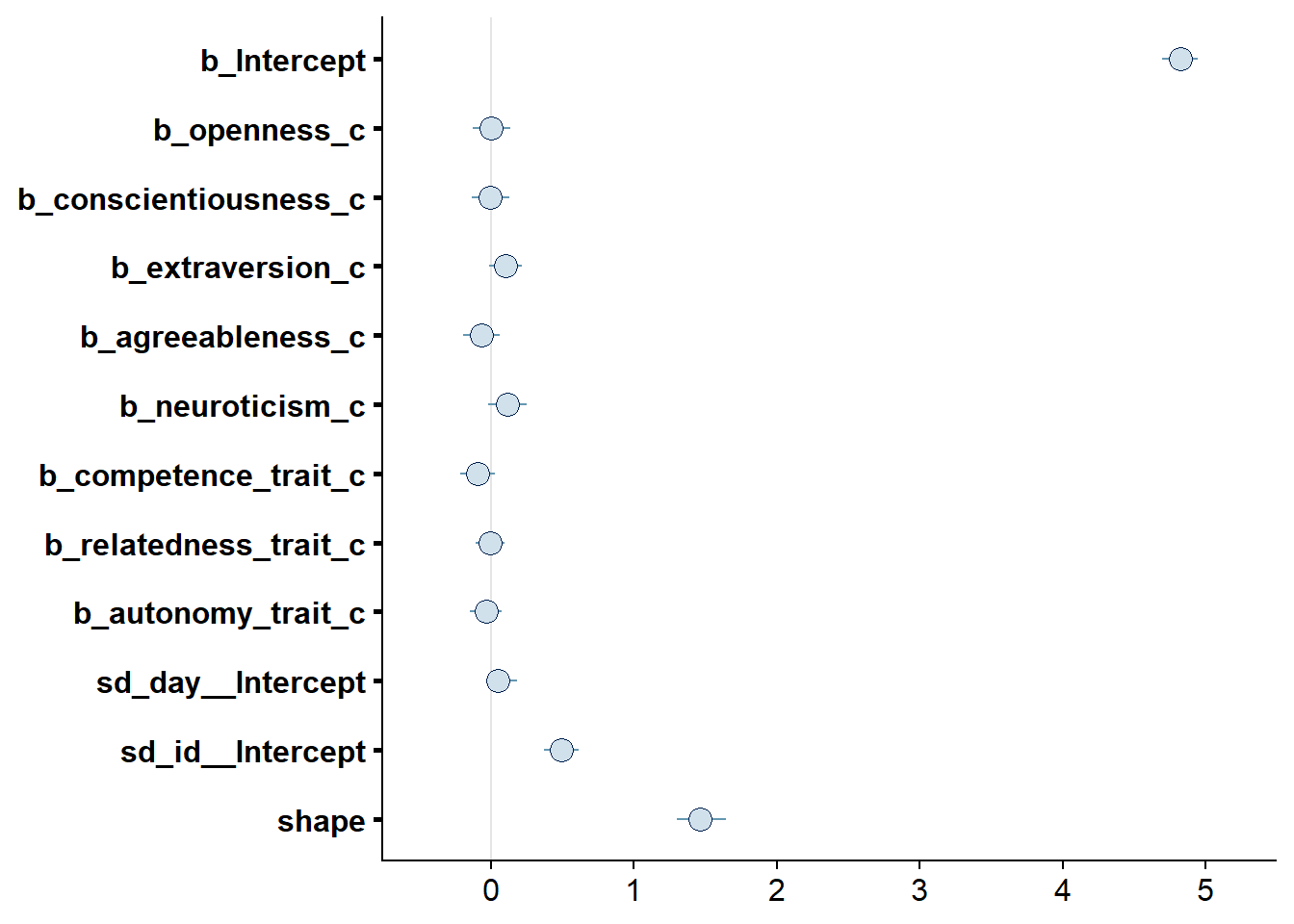

The effects plot (Figure 4.6) shows that visually, but also shows that the model does a fine job in describing the data, given the relatively (at least on the log scale) narrow 95% credible interval. Overall, there’s little evidence that personality traits are related so smartphone use, except for some tentative evidence that neurotic people use more social media and those who generally feel a level of competence in their lives use them less.

Figure 4.6: Effects plot for Model 1

4.3.2 Model 2: Trait variables predicting subjective use

Next up, I predict subjective use from the same predictors. We know that objective and subjective use aren’t perfectly correlated. Then again, the priors for Model 1 were only weakly regularizing, which is why I use the same priors again.

priors_model2 <- 
  c(
    # intercept
    prior(normal(4.5, 0.8), class = Intercept),
    
    # prior on effects
    prior(normal(0, 0.1), class = b),
    
    # all other effects
    prior(gamma(2.5, 100), class = shape)
  )

Alright, time to run the model. The subjective social media estimate had one missing value. Usually I’d impute missing values during model fitting, but with one, I think it’s safe to drop it.

model2 <- 
  brm(
    data = dat,
    family = Gamma(link = "log"),
    prior = priors_model2,
    social_media_subjective ~
      1 +
      openness_c +
      conscientiousness_c +
      extraversion_c +
      agreeableness_c +
      neuroticism_c +
      competence_trait_c +
      relatedness_trait_c +
      autonomy_trait_c +
      (1 | id) +
      (1 | day),
    iter = 5000,
    warmup = 2000,
    chains = 4,
    cores = 4,
    seed = 42,
    control = list(adapt_delta = 0.999),
    file = here("models", "model2")
  )

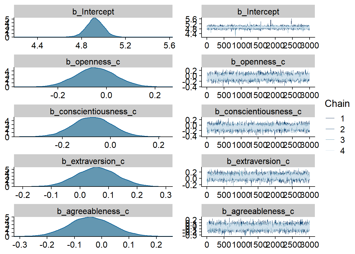
Let’s inspect the traceplots. Overall, they look fine and the chains seem to have mixed well (Figure ??). Again, everything looks fine.

Figure 4.7: Traceplots and posterior distributions for Model 2

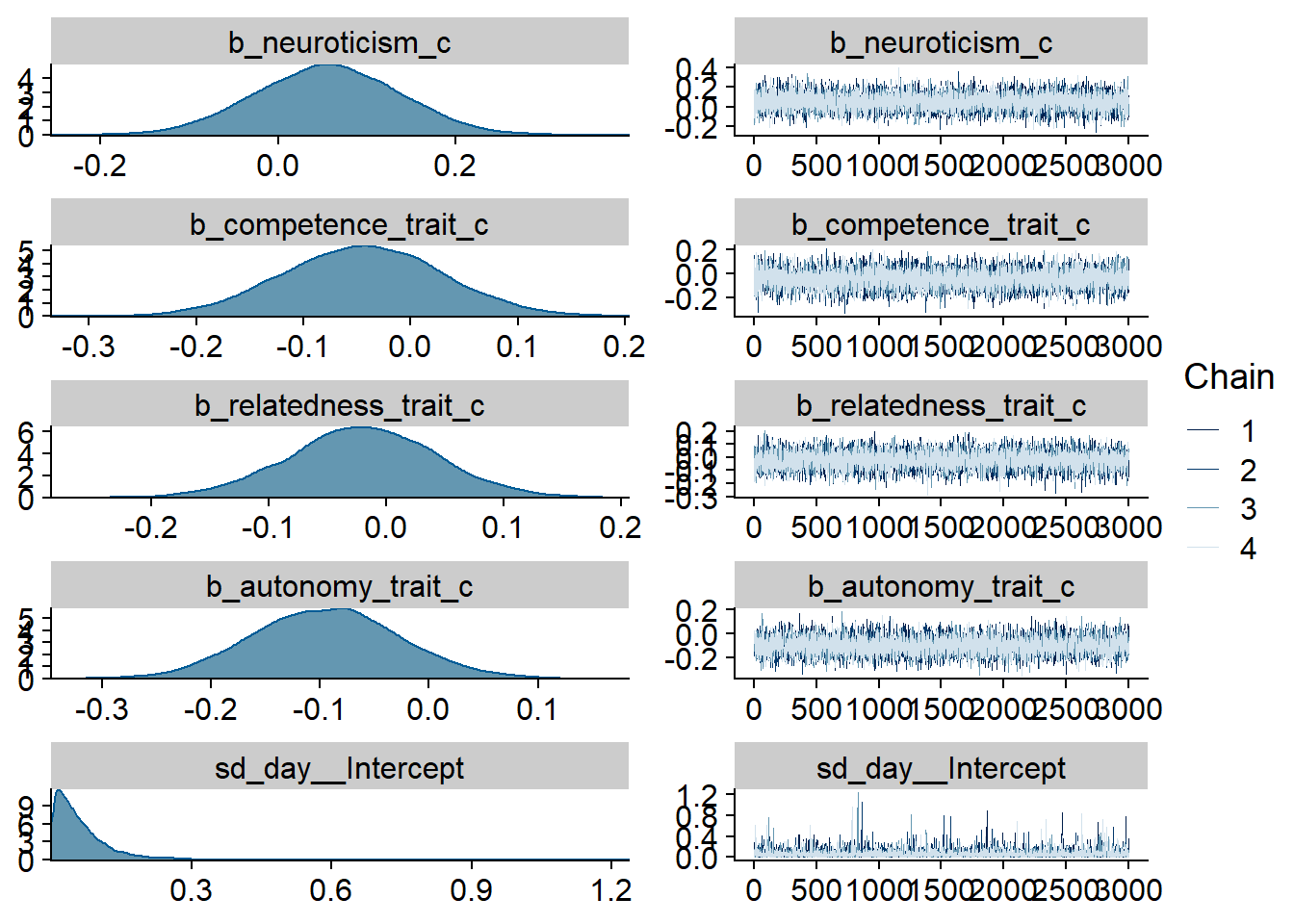
Figure 4.8: Traceplots and posterior distributions for Model 2

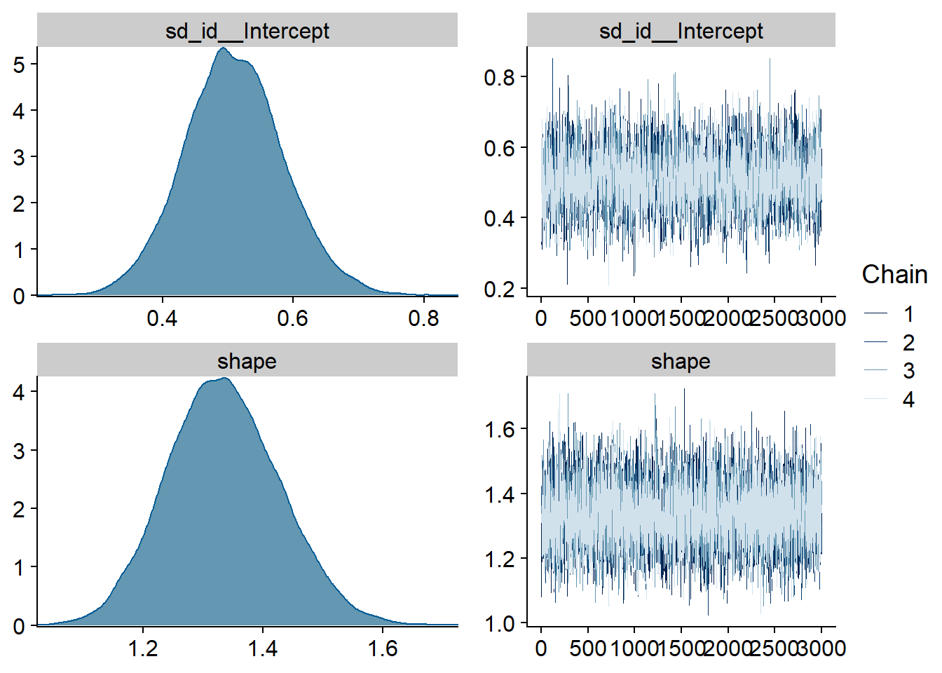
Figure 4.9: Traceplots and posterior distributions for Model 2

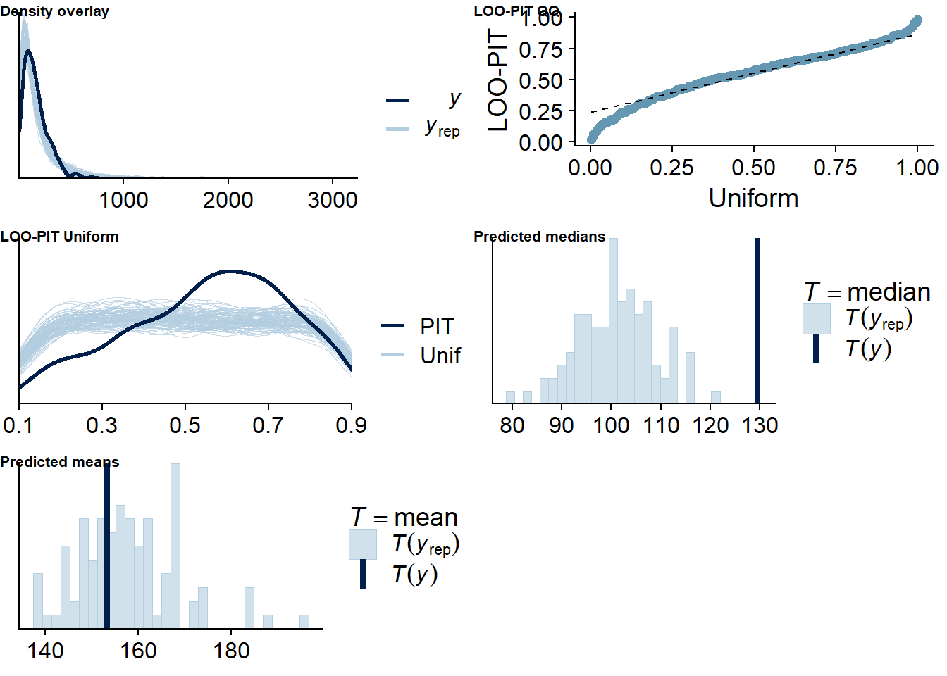
The posterior predictive distribution (Figure 4.10) looks similar to Model 1, with a tendency of the model to underestimate self-reported social media use. All other diagnostics look similar, which is not surprising given that the outcomes of Model 1 and Model 2 are correlated. Overall, the model fit is okay-ish, but certainly not excellent.

Figure 4.10: Posterior predictive checks for Model 2

Let’s again check for potentially influential values. The model diagnostics look good. Even though there were several rather large raw values on the outcome variable, the model expects them because we model the outcome as a Gamma distribution. We need to calculate ELPD directly, which shows no outliers.

loo(model2, reloo = TRUE)

## 1 problematic observation(s) found.
## The model will be refit 1 times.

## 
## Fitting model 1 out of 1 (leaving out observation 392)

## Start sampling

## 
## Computed from 12000 by 428 log-likelihood matrix
## 
##          Estimate   SE
## elpd_loo  -2502.2 15.9
## p_loo        24.6  1.6
## looic      5004.4 31.8
## ------
## Monte Carlo SE of elpd_loo is 0.1.
## 
## Pareto k diagnostic values:
##                          Count Pct.    Min. n_eff
## (-Inf, 0.5]   (good)     421   98.4%   412       
##  (0.5, 0.7]   (ok)         7    1.6%   2552      
##    (0.7, 1]   (bad)        0    0.0%   <NA>      
##    (1, Inf)   (very bad)   0    0.0%   <NA>      
## 
## All Pareto k estimates are ok (k < 0.7).
## See help('pareto-k-diagnostic') for details.

Alright, time to look at the summary. This time, all posterior distributions are mostly centered around zero, so we can be 95% (always conditional on the model) certain that personality traits and motivations are not meaningfully (i.e., large effect) related to self-reported social media use. Maybe autonomy gets close, but the posterior distributions still includes zero and small negative effects.

summary(model2, priors = TRUE)

##  Family: gamma 
##   Links: mu = log; shape = identity 
## Formula: social_media_subjective ~ 1 + openness_c + conscientiousness_c + extraversion_c + agreeableness_c + neuroticism_c + competence_trait_c + relatedness_trait_c + autonomy_trait_c + (1 | id) + (1 | day) 
##    Data: study1 (Number of observations: 428) 
## Samples: 4 chains, each with iter = 5000; warmup = 2000; thin = 1;
##          total post-warmup samples = 12000
## 
## Priors: 
## b ~ normal(0, 0.1)
## Intercept ~ normal(4.5, 0.8)
## sd ~ student_t(3, 0, 2.5)
## shape ~ gamma(2.5, 100)
## 
## Group-Level Effects: 
## ~day (Number of levels: 5) 
##               Estimate Est.Error l-95% CI u-95% CI Rhat Bulk_ESS Tail_ESS
## sd(Intercept)     0.07      0.07     0.00     0.25 1.00     5313     5290
## 
## ~id (Number of levels: 94) 
##               Estimate Est.Error l-95% CI u-95% CI Rhat Bulk_ESS Tail_ESS
## sd(Intercept)     0.51      0.08     0.36     0.66 1.00     3414     5977
## 
## Population-Level Effects: 
##                     Estimate Est.Error l-95% CI u-95% CI Rhat Bulk_ESS Tail_ESS
## Intercept               4.92      0.08     4.76     5.08 1.00     5160     5656
## openness_c             -0.04      0.08    -0.21     0.12 1.00     9524     8983
## conscientiousness_c    -0.08      0.08    -0.24     0.08 1.00     8766     9443
## extraversion_c          0.06      0.07    -0.08     0.20 1.00     7976     7997
## agreeableness_c        -0.04      0.08    -0.19     0.12 1.00     8628     8552
## neuroticism_c           0.06      0.08    -0.10     0.21 1.00     9739     9263
## competence_trait_c     -0.04      0.07    -0.19     0.10 1.00     8340     8625
## relatedness_trait_c    -0.02      0.06    -0.14     0.10 1.00     7666     7707
## autonomy_trait_c       -0.09      0.07    -0.22     0.04 1.00     7668     8591
## 
## Family Specific Parameters: 
##       Estimate Est.Error l-95% CI u-95% CI Rhat Bulk_ESS Tail_ESS
## shape     1.33      0.09     1.16     1.52 1.00     6185     9161
## 
## Samples were drawn using sampling(NUTS). For each parameter, Bulk_ESS
## and Tail_ESS are effective sample size measures, and Rhat is the potential
## scale reduction factor on split chains (at convergence, Rhat = 1).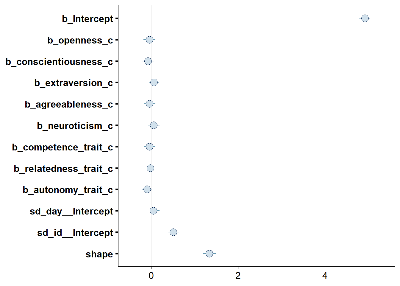

The effects plot (Figure 4.11) visually confirms that none of the predictors seem influential.

Figure 4.11: Effects plot for Model 2

4.3.3 Model 3: Trait variables predicting accuracy

For this model, it’s hard to choose informed priors, mainly because there’s no literature on the relation between personality traits and accuracy. Also, it’s unclear what distribution for accuracy we should expect prior to having seen the data. The few papers out there show that people generally overestimate their (social) media use, which would speak for centering the distribution on a positive value (i.e., positive error). Other than that, I’d expect a normal distribution, quite likely with fat tails, and possibly right skewed. Therefore, I’ll use a student-t distribution outcome family. I start with a t distribution as prior for the intercept that is slightly centered on overestimates (i.e., 20%), but with quite some potential for extreme values and fairly fat tails. See Figure 4.12 left panel, for a visualization.

As for the effects of the personality traits, I’ll be skeptical of any effects and thus use weakly regularizing normal priors that are centered on zero, with a small range for the effect: If a person goes from average on a trait to one above average, we’d expect that 95% of the effects should be between -50% and +50% (i.e., SD of 25). See the right panel in the figure below for a visualization.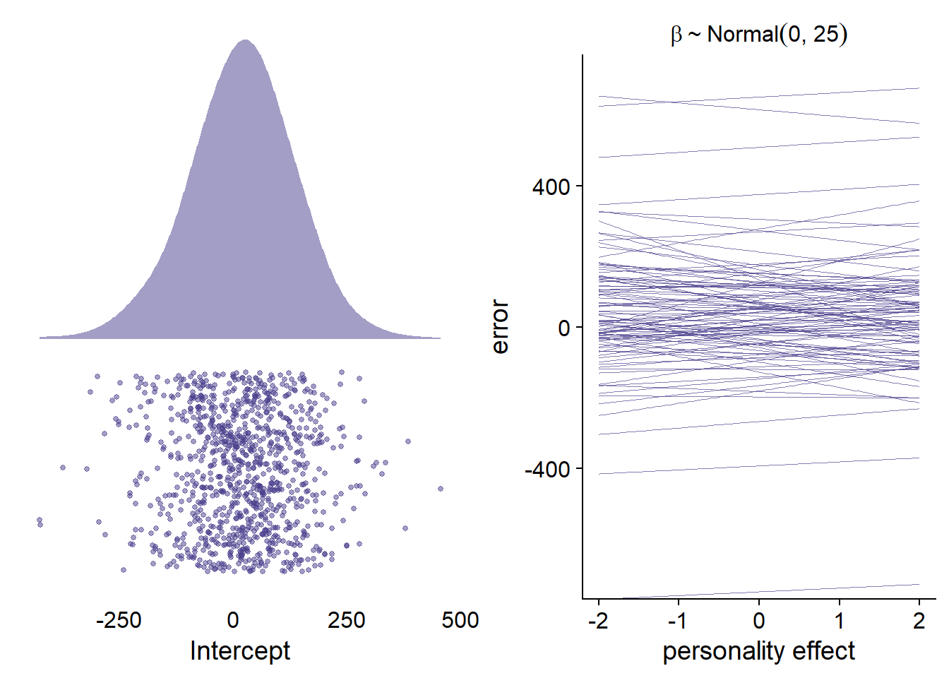

Figure 4.12: Prior simmulations for Model 2

Then let’s set those priors we simulated above.

priors_model3 <- 
  c(
    # intercept
    prior(student_t(10, 20, 100), class = Intercept),
    
    # all other effects
    prior(normal(0, 25), class = b)
  )

error had 53 missing values. Again, with such few cases, I’m fine with dropping those during model fitting.

model3 <- 
  brm(
    data = dat,
    family = student,
    prior = priors_model3,
    error ~
      1 +
      openness_c +
      conscientiousness_c +
      extraversion_c +
      agreeableness_c +
      neuroticism_c +
      competence_trait_c +
      relatedness_trait_c +
      autonomy_trait_c +
      (1 | id) +
      (1 | day),
    iter = 5000,
    warmup = 2000,
    chains = 4,
    cores = 4,
    seed = 42,
    control = list(adapt_delta = 0.99),
    file = here("models", "model3")
  )

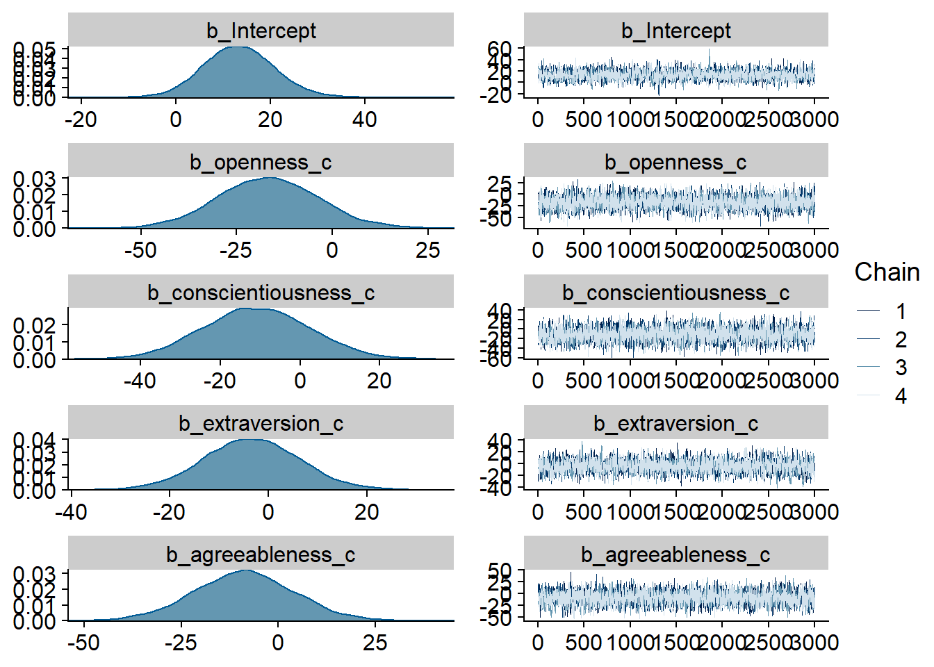
Overall, the traceplots look fine and the chains seem to have mixed well, see (Figure ??). Again, the variance around the residuals for the day grouping is estimated to be small and zero often.

Figure 4.13: Traceplots and posterior distributions for Model 3

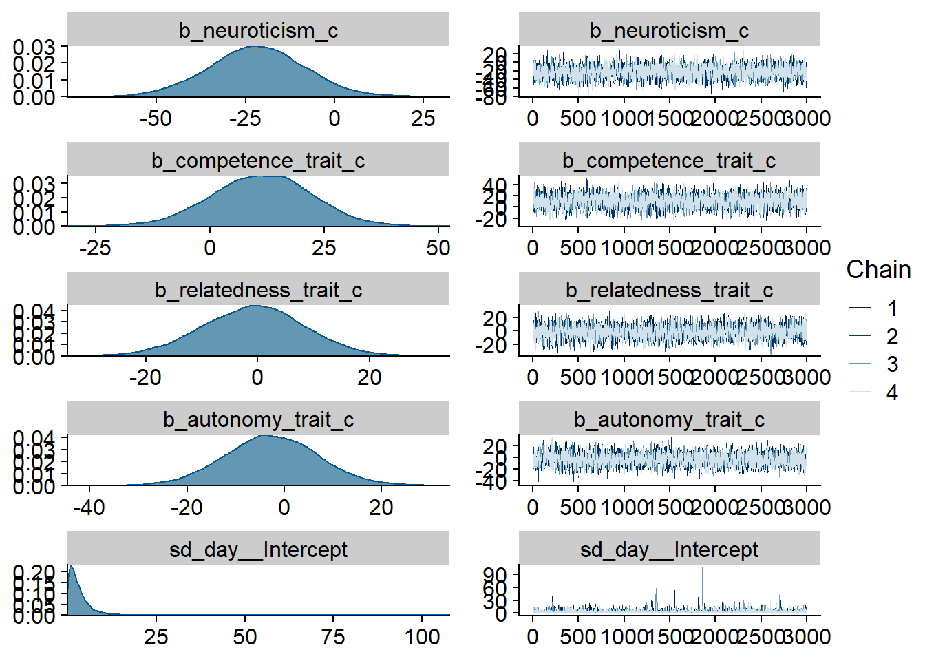
Figure 4.14: Traceplots and posterior distributions for Model 3

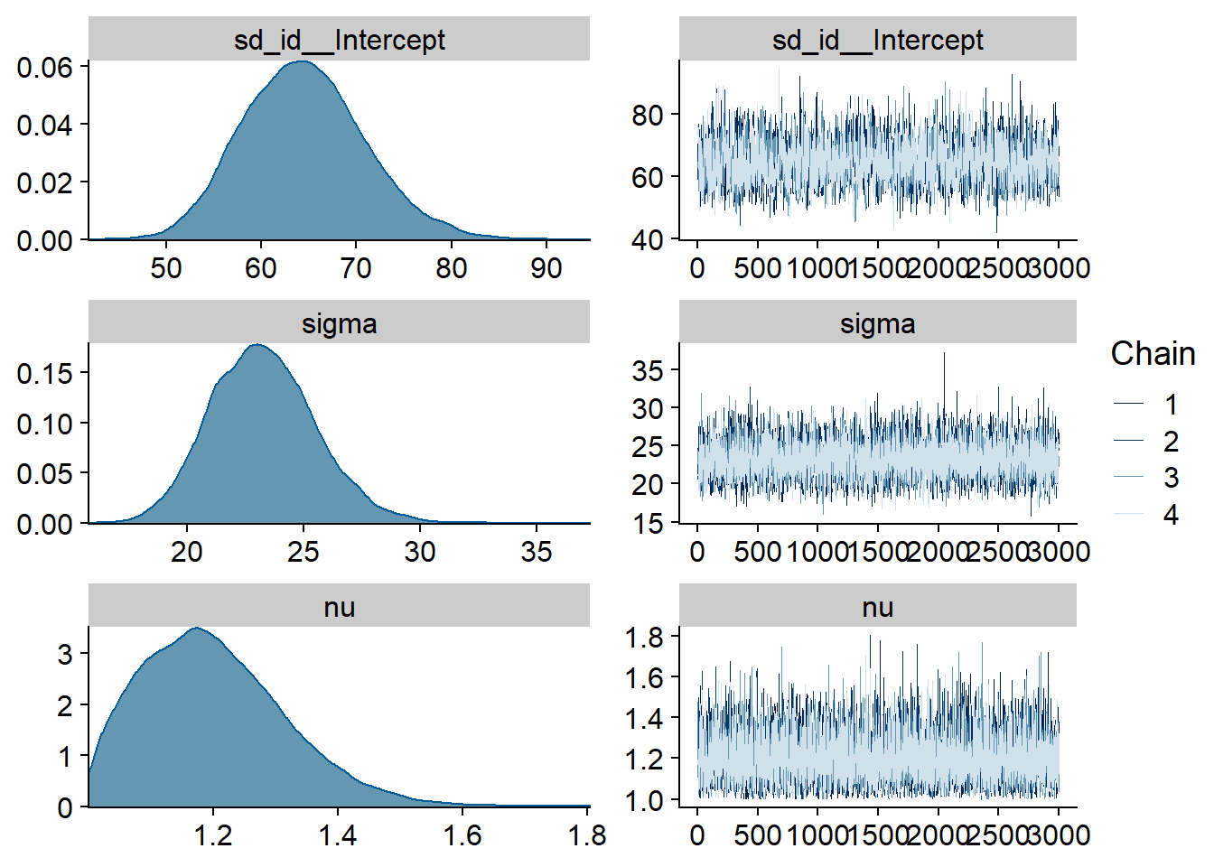
Figure 4.15: Traceplots and posterior distributions for Model 3

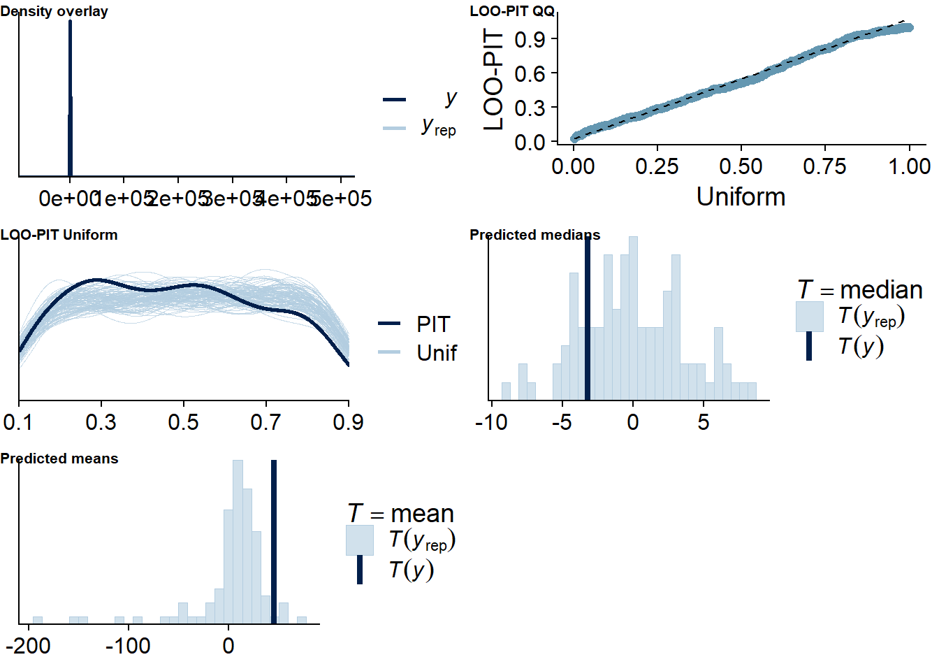
The posterior predictive checks (Figure ??) look good. Note that the upper left panel looks strange because of the massive scale on the x-axis, which is why I reproduce it again at the bottom. We see that the student t distribution assigns too much posterior mass to negative values, whereas the data are right skewed. For even better fit, we might think about fitting a skew-normal outcome distribution, but I’d say that the student-t was most appropriate before seeing the data. We see that the current models does an okay job in recovering the mean and the median.

Figure 4.16: Posterior predictive checks for Model 3

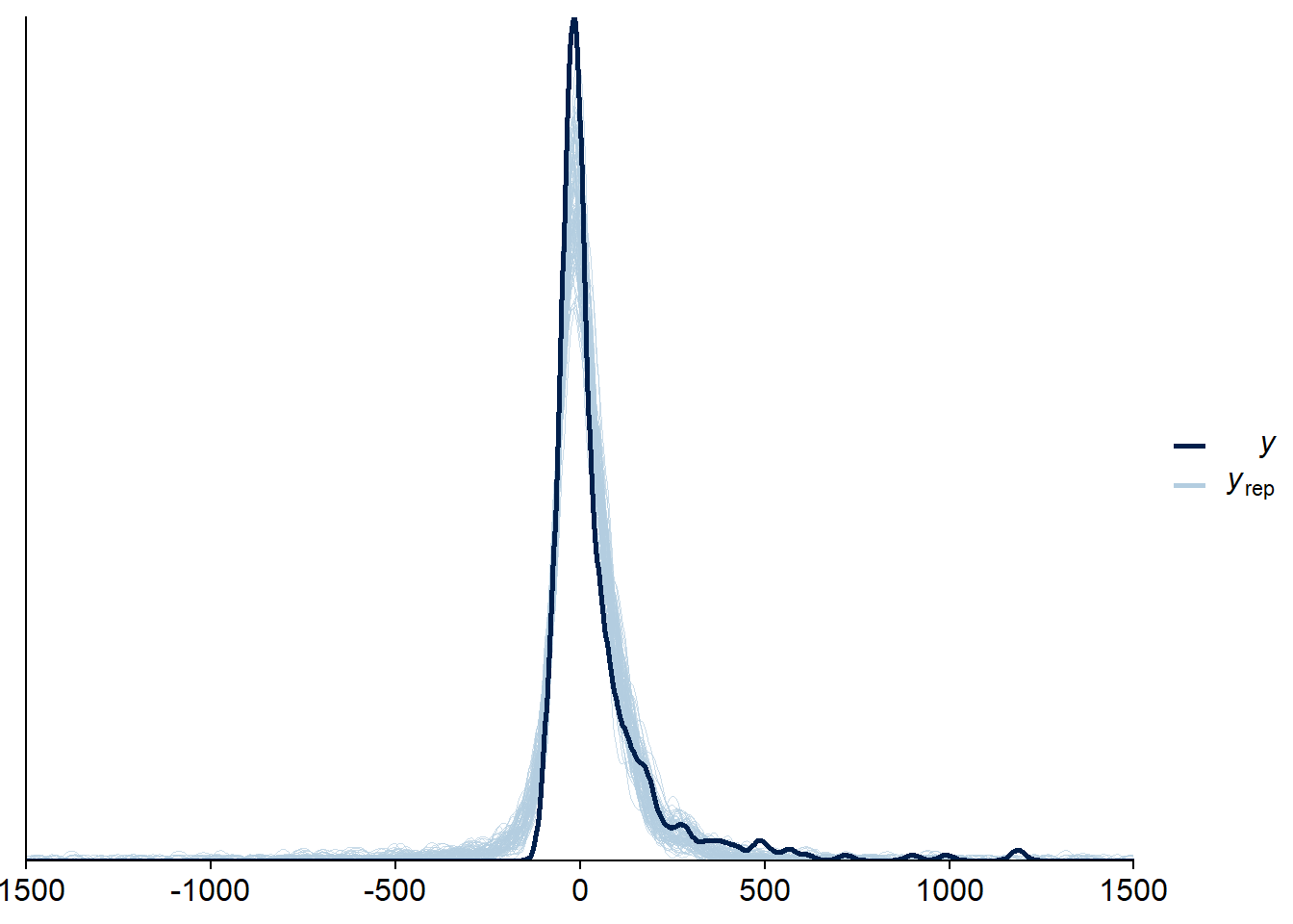
Figure 4.17: Posterior predictive checks for Model 3

Let’s again check for potentially influential values. Three potentially influential cases are flagged, which is why we calculate them precisely by setting reloo to TRUE. When we calculate ELPD directly, all values appear unproblematic. The results seem trustworthy.

loo(model3, reloo = TRUE)

## 3 problematic observation(s) found.
## The model will be refit 3 times.

## 
## Fitting model 1 out of 3 (leaving out observation 40)

## 
## Fitting model 2 out of 3 (leaving out observation 43)

## 
## Fitting model 3 out of 3 (leaving out observation 111)

## Start sampling
## Start sampling
## Start sampling

## 
## Computed from 12000 by 426 log-likelihood matrix
## 
##          Estimate   SE
## elpd_loo  -2415.2 31.4
## p_loo       136.1  6.7
## looic      4830.3 62.7
## ------
## Monte Carlo SE of elpd_loo is 0.2.
## 
## Pareto k diagnostic values:
##                          Count Pct.    Min. n_eff
## (-Inf, 0.5]   (good)     421   98.8%   436       
##  (0.5, 0.7]   (ok)         5    1.2%   714       
##    (0.7, 1]   (bad)        0    0.0%   <NA>      
##    (1, Inf)   (very bad)   0    0.0%   <NA>      
## 
## All Pareto k estimates are ok (k < 0.7).
## See help('pareto-k-diagnostic') for details.

Let’s inspect the summary. There doesn’t seem to be much going on when it comes to the predictors. For all predictors, we cannot be 95% certain that zero isn’t the true effect (conditional on the model). Again, neuroticism comes close.

summary(model3, priors = TRUE)

##  Family: student 
##   Links: mu = identity; sigma = identity; nu = identity 
## Formula: error ~ 1 + openness_c + conscientiousness_c + extraversion_c + agreeableness_c + neuroticism_c + competence_trait_c + relatedness_trait_c + autonomy_trait_c + (1 | id) + (1 | day) 
##    Data: study1 (Number of observations: 426) 
## Samples: 4 chains, each with iter = 5000; warmup = 2000; thin = 1;
##          total post-warmup samples = 12000
## 
## Priors: 
## b ~ normal(0, 25)
## Intercept ~ student_t(10, 20, 100)
## nu ~ gamma(2, 0.1)
## sd ~ student_t(3, 0, 57.7)
## sigma ~ student_t(3, 0, 57.7)
## 
## Group-Level Effects: 
## ~day (Number of levels: 5) 
##               Estimate Est.Error l-95% CI u-95% CI Rhat Bulk_ESS Tail_ESS
## sd(Intercept)     3.21      3.59     0.11    11.79 1.00     5317     5339
## 
## ~id (Number of levels: 94) 
##               Estimate Est.Error l-95% CI u-95% CI Rhat Bulk_ESS Tail_ESS
## sd(Intercept)    64.47      6.40    52.80    77.92 1.00     2251     3791
## 
## Population-Level Effects: 
##                     Estimate Est.Error l-95% CI u-95% CI Rhat Bulk_ESS Tail_ESS
## Intercept              13.34      7.62    -1.10    28.66 1.00     2110     4056
## openness_c            -16.81     13.17   -42.62     9.80 1.00     2867     4647
## conscientiousness_c   -10.92     13.30   -36.68    15.14 1.00     2861     5033
## extraversion_c         -3.45      9.78   -22.74    16.05 1.00     2531     4145
## agreeableness_c        -8.85     12.86   -34.32    16.69 1.00     2758     4088
## neuroticism_c         -21.89     13.39   -48.27     4.58 1.00     2828     4561
## competence_trait_c     11.31     10.95   -10.34    32.57 1.00     2710     4601
## relatedness_trait_c    -0.79      9.09   -18.85    16.70 1.00     2056     3941
## autonomy_trait_c       -2.66      9.59   -21.25    16.33 1.00     2594     4595
## 
## Family Specific Parameters: 
##       Estimate Est.Error l-95% CI u-95% CI Rhat Bulk_ESS Tail_ESS
## sigma    23.26      2.23    19.16    27.85 1.00     5374     7711
## nu        1.20      0.11     1.02     1.46 1.00     5581     4487
## 
## Samples were drawn using sampling(NUTS). For each parameter, Bulk_ESS
## and Tail_ESS are effective sample size measures, and Rhat is the potential
## scale reduction factor on split chains (at convergence, Rhat = 1).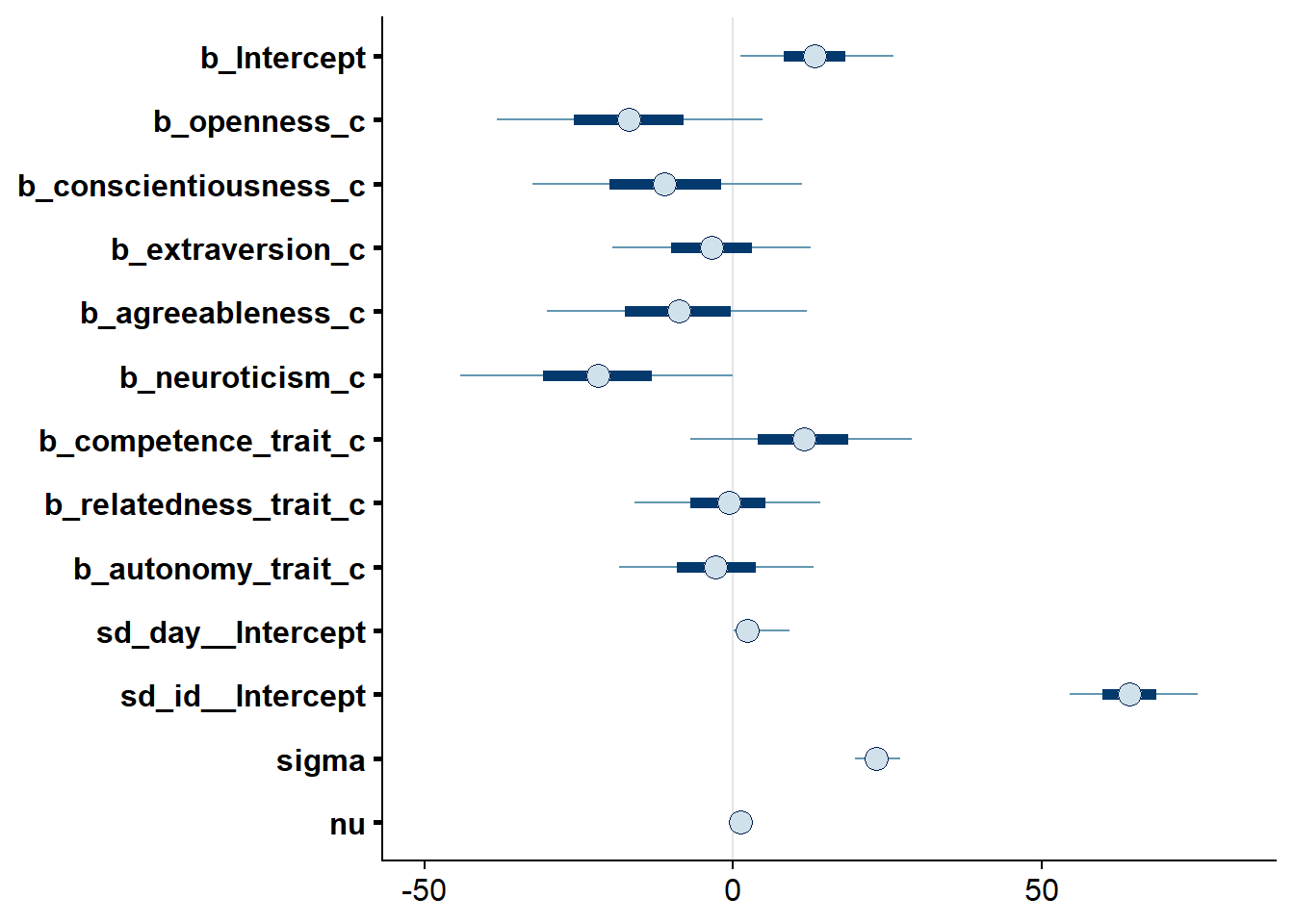

The effects plot (Figure 4.18) visually confirms that none of the predictors seem largely influential. If anything, it appears neurotic people might underestimate their social media use, but again their interval contains zero.

Figure 4.18: Effects plot for Model 3

4.4 Do state (i.e., day-level) variables predict social media use and accuracy?

For the next section, we look at whether day-level variables (i.e., variables reported during experience sampling) predict subjective use, objective use, and accuracy. Again, we have three questions:

Do day-level variables predict objective-only engagement?
Do day-level variables predict subjective-only engagement?
Do day-level variables predict accuracy?

Once more I’ll construct a model for each of those three questions. Our dependent variables are the same as in the previous block of models: social_media_objective, social_media_subjective, and error.

Our predictors will be variables on the day-level, so state variables: need satisfaction for autonomy, competence, and relatedness as well as four experiential qualities during participants’ days (boredom, enjoyment, satisfaction, and stress).

Because we want to separate between-person and within-person effects, we’ll do group-mean centering (i.e., per participant) and the calculate the deviation of each observation from that group mean. We enter both the person mean and their deviation as predictors, which will lead to a lot of variables, because each of the seven predictors will be separated into a between-person and a within-person predictor. See this blogpost for a tutorial on centering.

dat <- 
  dat %>% 
  group_by(id) %>% 
  mutate(
    across(
      c(autonomy_state:relatedness_state, satisfied:enjoyable),
      list(
        between = ~ mean(.x, na.rm = TRUE),
        within = ~.x - mean(.x, na.rm = TRUE)
      )
    )
  ) %>% 
  ungroup()

4.4.1 Model 4: State variables predicting objective use

First, I choose sensible priors. In contrast to previous models, there isn’t much literature that could inform priors on our predictors. The same goes for the experiential qualities. We’ll go with a “maximal” model where each participant and day get their own intercept plus random slopes nested within participant, because it’s plausible that the effects vary per participant. They could also vary by day, but a) there was little to no variation for day in previous models, and b) that would lead to more parameters than our little data could handle. Just like before we assume a Gamma distribution for the social media variables.

I’ll go step-by-step:

For the intercepts, I use the same prior as above in Models 1 and 2.
For basic psychological needs fixed effects, this paper reports very small relations between self-determined motivations at work and social media use (\(\beta\) < .06). However, most of the literature focuses on those motivations and social media addiction, enjoyment of social media, or satisfaction with social media. Therefore, I’ll use weakly regularizing priors for those effects, which means I’ll go with the same prior for the effects as for Models 1 and 2. I would expect larger differences on the between-level, based on the literature on media use and well-being. However, we don’t have that info for our predictors and the priors are rather weak, so I’ll apply them to both between and within predictors.
For the experiential qualities, there isn’t much literature out there that would allow choosing an informed prior. Most of those experiential qualities are about having a fulfilled and good day, which taps into the whole controversy over the relation between such experiences and social media. Therefore, I’ll take a skeptical stance here and again assign the same weakly regularizing priors (aka the priors we also used for Models 1 and 2).
For the variances (sigmas) I’ll take the brms default priors because I have no prior information, nor how the effects vary across day and participant.
For the correlation between intercepts and slopes, I’ll again use the default prior, mostly because those have shown to help with convergence and I don’t have good information on which correlation to expect.

priors_model4 <- 
  c(
    # intercept
    prior(normal(4.5, 0.8), class = Intercept),
    
    # prior on effects
    prior(normal(0, 0.1), class = b),
    
    # prior on shape
    prior(gamma(2.5, 100), class = shape)
  )

Let’s run the model. Note that the within-deviations can vary per participant, but not the between effects.

model4 <- 
  brm(
    data = dat,
    family = Gamma(link = "log"),
    prior = priors_model4,
    social_media_objective ~
      1 +
      autonomy_state_between +
      competence_state_between +
      relatedness_state_between +
      satisfied_between +
      boring_between +
      stressful_between +
      enjoyable_between +
      autonomy_state_within +
      competence_state_within +
      relatedness_state_within +
      satisfied_within +
      boring_within +
      stressful_within +
      enjoyable_within +
      (
        1 +
        autonomy_state_within +
        competence_state_within +
        relatedness_state_within +
        satisfied_within +
        boring_within +
        stressful_within +
        enjoyable_within |
        id
      ) +
      (1 |day),
    iter = 5000,
    warmup = 2000,
    chains = 4,
    cores = 4,
    seed = 42,
    control = list(
      adapt_delta = 0.99
    ),
    file = here("models", "model4")
  )

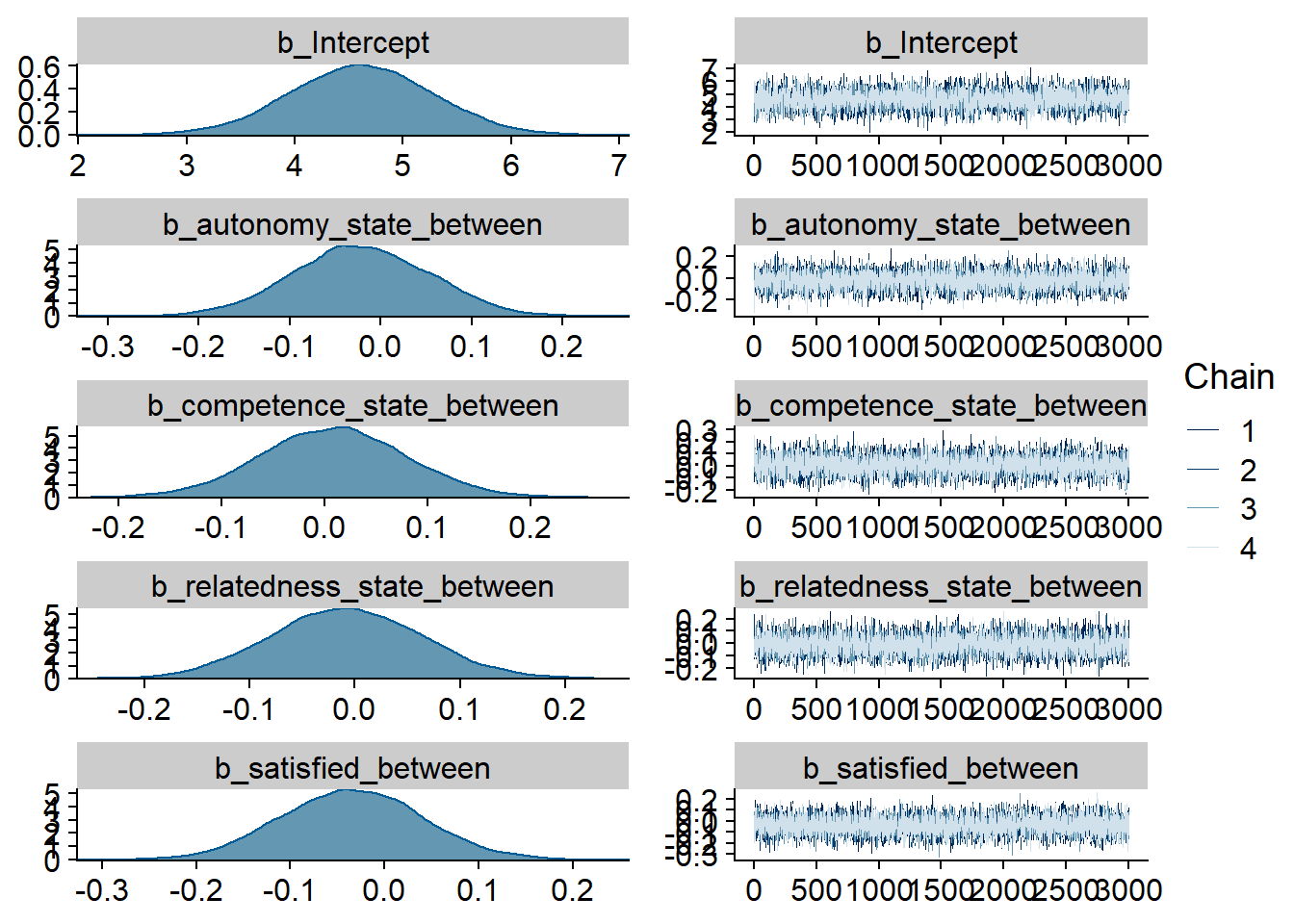
Overall, the traceplots look fine and the chains seem to have mixed well (Figure ??). Again the variance around the day grouping is small and mostly estimated to be zero or close to zero.

Figure 4.19: Traceplots and posterior distributions for Model 4

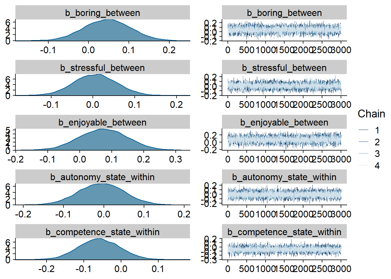
Figure 4.20: Traceplots and posterior distributions for Model 4

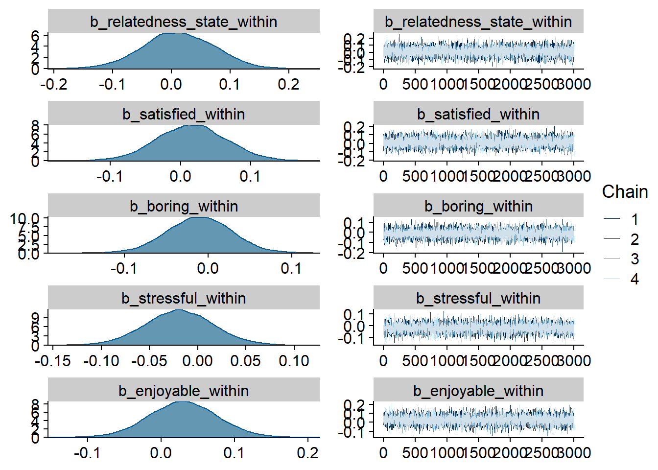
Figure 4.21: Traceplots and posterior distributions for Model 4

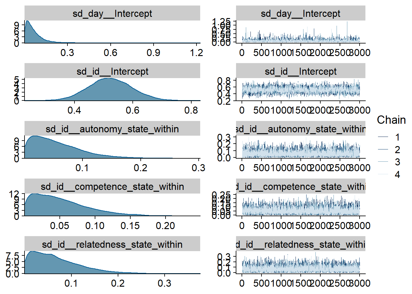
Figure 4.22: Traceplots and posterior distributions for Model 4

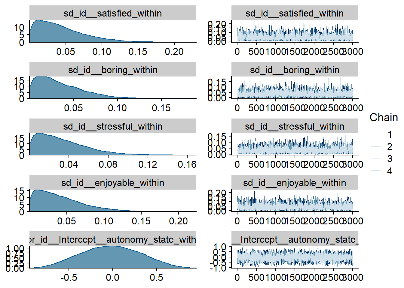
Figure 4.23: Traceplots and posterior distributions for Model 4

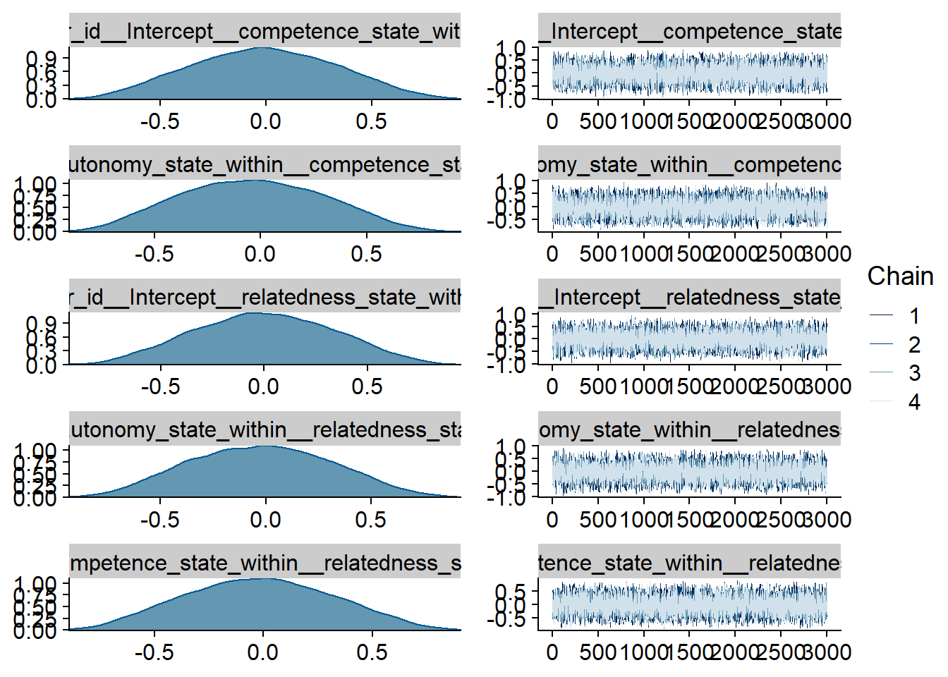
Figure 4.24: Traceplots and posterior distributions for Model 4

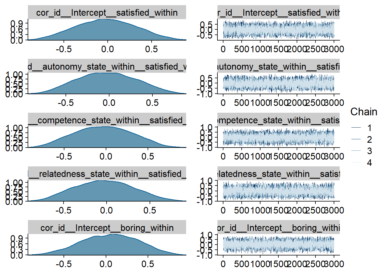
Figure 4.25: Traceplots and posterior distributions for Model 4

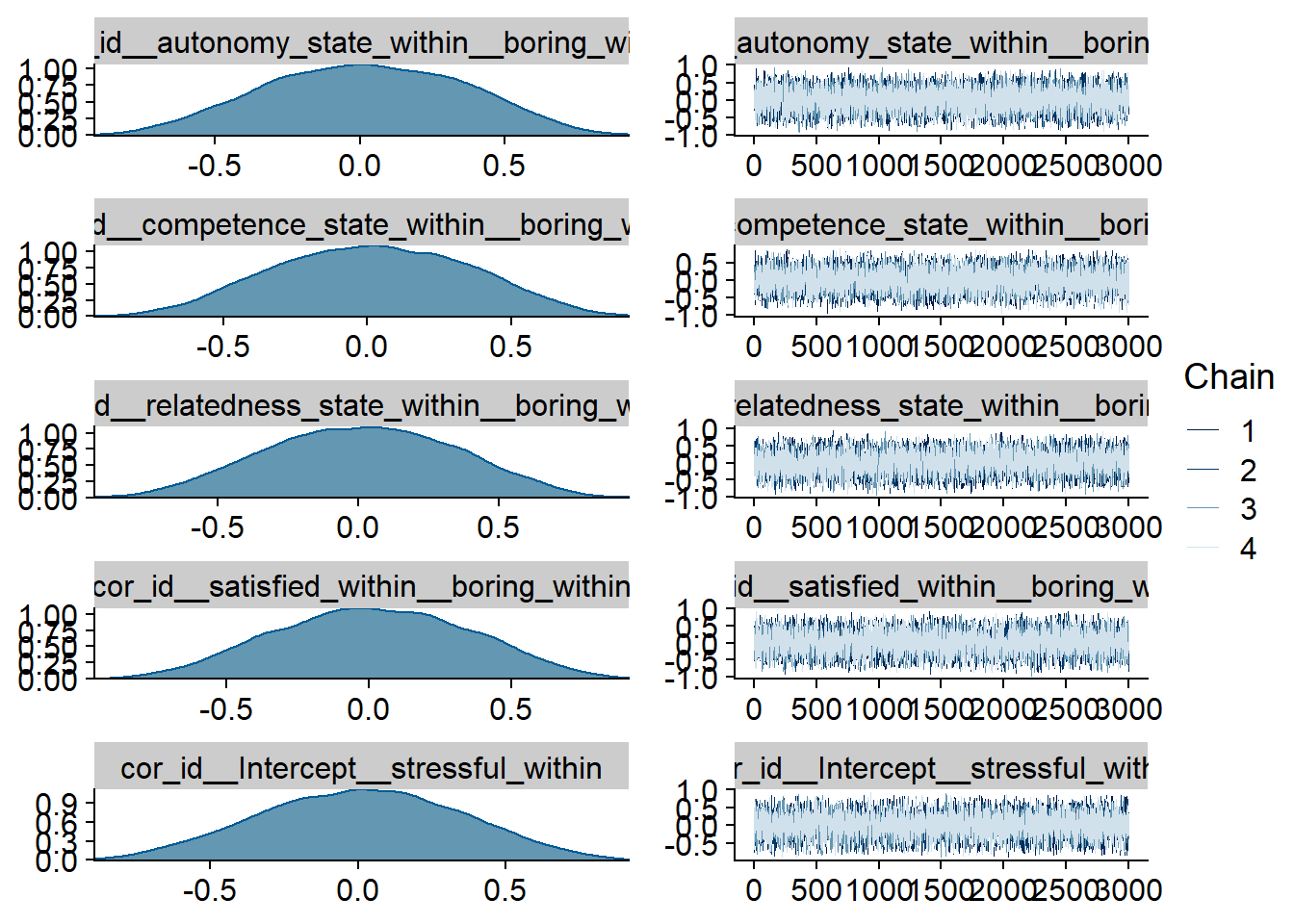
Figure 4.26: Traceplots and posterior distributions for Model 4

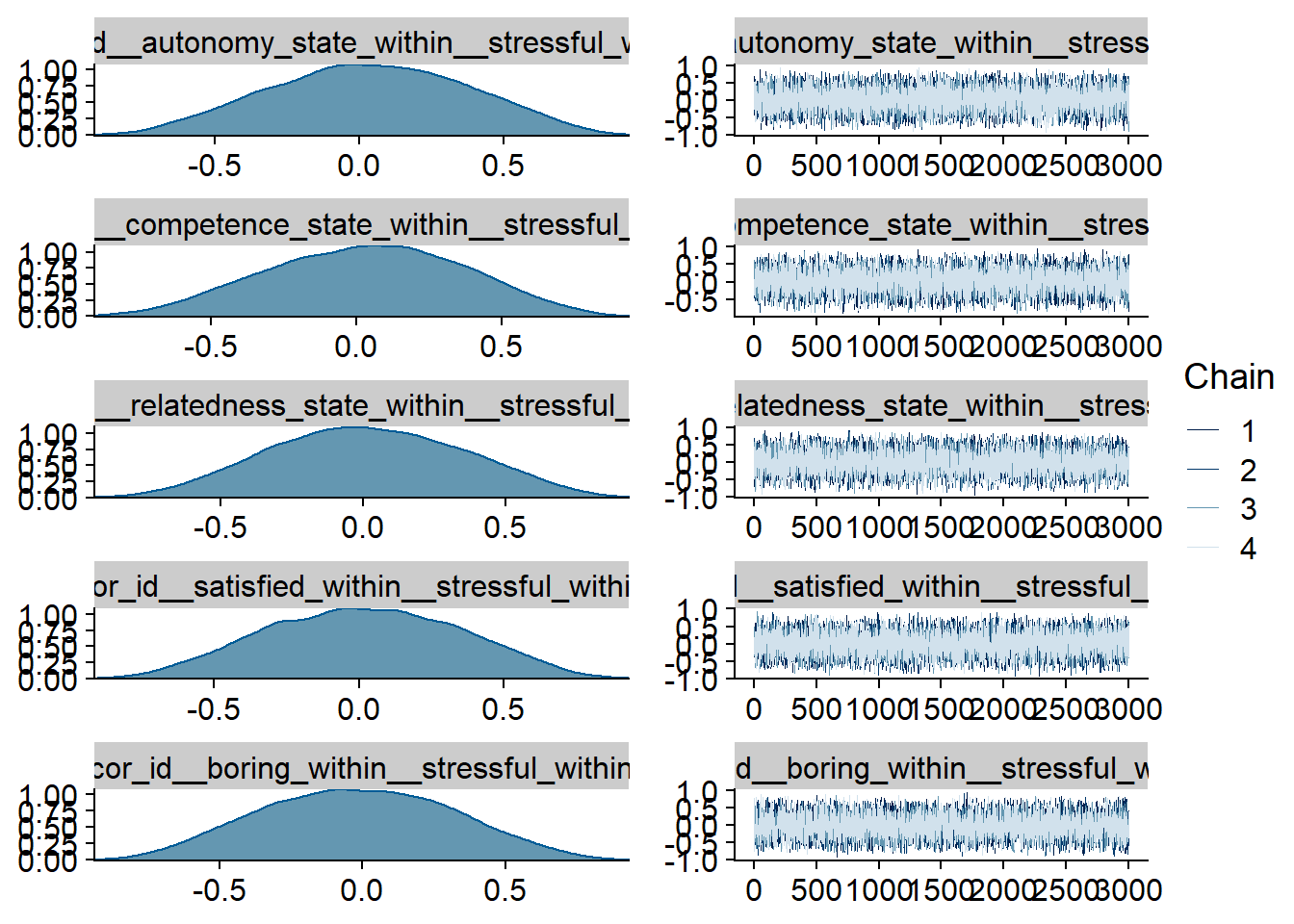
Figure 4.27: Traceplots and posterior distributions for Model 4

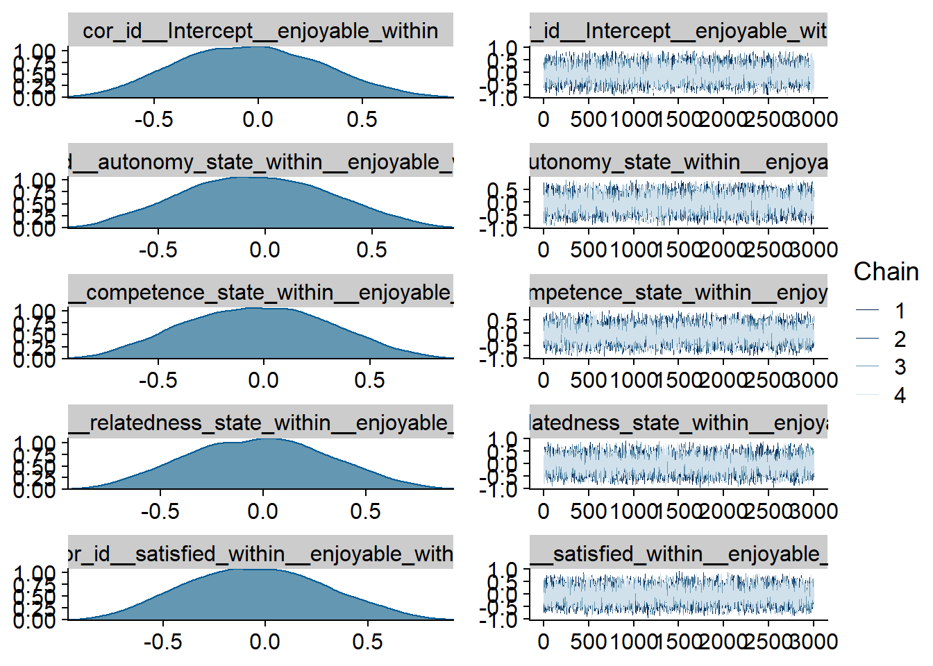
Figure 4.28: Traceplots and posterior distributions for Model 4

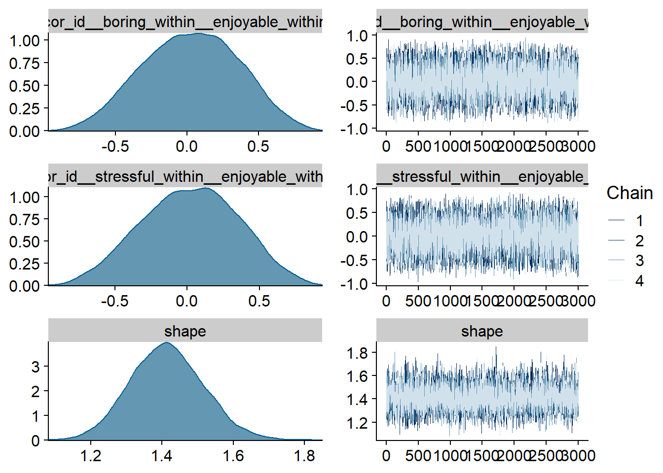
Figure 4.29: Traceplots and posterior distributions for Model 4

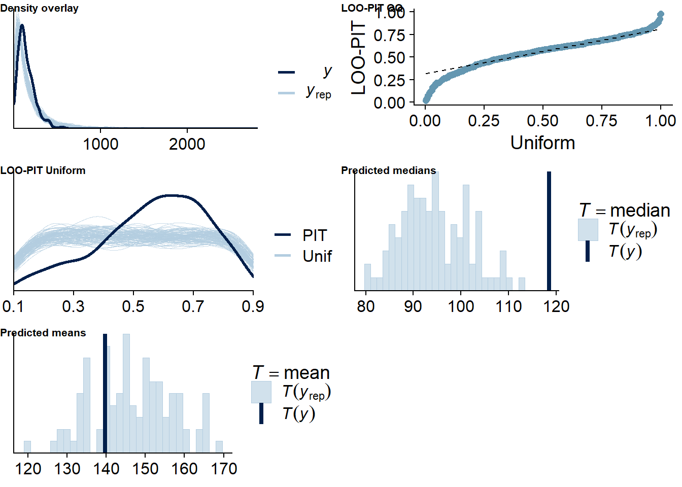
The posterior predictive check shows that the model does a mediocre job. The model does a good job retrieving the mean, but underestimates social media use once more. Also, the LOO-PIT diagnostics look like a different distribution will fit better, potentially a skewed normal or beta-distribution.

Figure 4.30: Posterior predictive checks for Model 4

Next, we check for potentially influential cases. There are none.

loo(model4)

## 
## Computed from 12000 by 420 log-likelihood matrix
## 
##          Estimate   SE
## elpd_loo  -2412.8 14.1
## p_loo        25.6  1.6
## looic      4825.6 28.1
## ------
## Monte Carlo SE of elpd_loo is 0.1.
## 
## Pareto k diagnostic values:
##                          Count Pct.    Min. n_eff
## (-Inf, 0.5]   (good)     408   97.1%   4830      
##  (0.5, 0.7]   (ok)        12    2.9%   1078      
##    (0.7, 1]   (bad)        0    0.0%   <NA>      
##    (1, Inf)   (very bad)   0    0.0%   <NA>      
## 
## All Pareto k estimates are ok (k < 0.7).
## See help('pareto-k-diagnostic') for details.

Let’s inspect the summary. There doesn’t seem to be much going on when it comes to the predictors.

summary(model4, priors = TRUE)

##  Family: gamma 
##   Links: mu = log; shape = identity 
## Formula: social_media_objective ~ 1 + autonomy_state_between + competence_state_between + relatedness_state_between + satisfied_between + boring_between + stressful_between + enjoyable_between + autonomy_state_within + competence_state_within + relatedness_state_within + satisfied_within + boring_within + stressful_within + enjoyable_within + (1 + autonomy_state_within + competence_state_within + relatedness_state_within + satisfied_within + boring_within + stressful_within + enjoyable_within | id) + (1 | day) 
##    Data: study1 (Number of observations: 420) 
## Samples: 4 chains, each with iter = 5000; warmup = 2000; thin = 1;
##          total post-warmup samples = 12000
## 
## Priors: 
## b ~ normal(0, 0.1)
## Intercept ~ normal(4.5, 0.8)
## L ~ lkj_corr_cholesky(1)
## sd ~ student_t(3, 0, 2.5)
## shape ~ gamma(2.5, 100)
## 
## Group-Level Effects: 
## ~day (Number of levels: 5) 
##               Estimate Est.Error l-95% CI u-95% CI Rhat Bulk_ESS Tail_ESS
## sd(Intercept)     0.07      0.07     0.00     0.25 1.00     5832     6519
## 
## ~id (Number of levels: 94) 
##                                                       Estimate Est.Error l-95% CI u-95% CI Rhat Bulk_ESS Tail_ESS
## sd(Intercept)                                             0.52      0.08     0.38     0.67 1.00     3573     5944
## sd(autonomy_state_within)                                 0.05      0.04     0.00     0.16 1.00     8320     5372
## sd(competence_state_within)                               0.05      0.04     0.00     0.14 1.00     8935     5381
## sd(relatedness_state_within)                              0.07      0.05     0.00     0.19 1.00     7787     4916
## sd(satisfied_within)                                      0.04      0.03     0.00     0.12 1.00     8933     5890
## sd(boring_within)                                         0.03      0.03     0.00     0.10 1.00     9702     5442
## sd(stressful_within)                                      0.03      0.02     0.00     0.09 1.00     9082     6157
## sd(enjoyable_within)                                      0.04      0.03     0.00     0.12 1.00     9115     5934
## cor(Intercept,autonomy_state_within)                     -0.02      0.33    -0.65     0.61 1.00    16387     8961
## cor(Intercept,competence_state_within)                   -0.01      0.34    -0.64     0.63 1.00    21044     9001
## cor(autonomy_state_within,competence_state_within)       -0.04      0.34    -0.66     0.60 1.00    13676     9802
## cor(Intercept,relatedness_state_within)                   0.00      0.33    -0.62     0.63 1.00    20886     8610
## cor(autonomy_state_within,relatedness_state_within)      -0.02      0.33    -0.65     0.61 1.00    14368     8242
## cor(competence_state_within,relatedness_state_within)    -0.02      0.33    -0.65     0.62 1.00    11400     8640
## cor(Intercept,satisfied_within)                          -0.02      0.33    -0.65     0.62 1.00    19647     8386
## cor(autonomy_state_within,satisfied_within)              -0.03      0.33    -0.65     0.62 1.00    13873     8112
## cor(competence_state_within,satisfied_within)            -0.03      0.34    -0.66     0.60 1.00    11687     9023
## cor(relatedness_state_within,satisfied_within)           -0.03      0.33    -0.65     0.62 1.00    10544     9670
## cor(Intercept,boring_within)                              0.05      0.33    -0.60     0.67 1.00    21420     8481
## cor(autonomy_state_within,boring_within)                  0.02      0.34    -0.62     0.64 1.00    16012     9390
## cor(competence_state_within,boring_within)                0.02      0.33    -0.61     0.64 1.00    12124     9240
## cor(relatedness_state_within,boring_within)               0.01      0.33    -0.62     0.63 1.00     9880     9056
## cor(satisfied_within,boring_within)                       0.01      0.34    -0.63     0.64 1.00     9165     9884
## cor(Intercept,stressful_within)                           0.01      0.33    -0.63     0.64 1.00    18727     8771
## cor(autonomy_state_within,stressful_within)               0.04      0.34    -0.61     0.66 1.00    14611     8703
## cor(competence_state_within,stressful_within)             0.03      0.33    -0.62     0.65 1.00    11626     9342
## cor(relatedness_state_within,stressful_within)            0.01      0.33    -0.62     0.65 1.00    10591     9391
## cor(satisfied_within,stressful_within)                    0.01      0.33    -0.62     0.64 1.00     8292     9818
## cor(boring_within,stressful_within)                      -0.02      0.33    -0.64     0.62 1.00     8189     9968
## cor(Intercept,enjoyable_within)                          -0.04      0.33    -0.66     0.62 1.00    19274     7944
## cor(autonomy_state_within,enjoyable_within)              -0.04      0.34    -0.68     0.62 1.00    13860     8987
## cor(competence_state_within,enjoyable_within)            -0.03      0.34    -0.66     0.61 1.00    11180     8545
## cor(relatedness_state_within,enjoyable_within)           -0.02      0.34    -0.65     0.63 1.00     9846     9047
## cor(satisfied_within,enjoyable_within)                   -0.05      0.33    -0.66     0.61 1.00     8402     9749
## cor(boring_within,enjoyable_within)                       0.03      0.33    -0.61     0.65 1.00     7006     9546
## cor(stressful_within,enjoyable_within)                    0.02      0.33    -0.63     0.64 1.00     7054     9355
## 
## Population-Level Effects: 
##                           Estimate Est.Error l-95% CI u-95% CI Rhat Bulk_ESS Tail_ESS
## Intercept                     4.61      0.66     3.32     5.89 1.00     7471     8345
## autonomy_state_between       -0.02      0.08    -0.17     0.12 1.00     9979     9622
## competence_state_between      0.01      0.07    -0.13     0.15 1.00     9383    10215
## relatedness_state_between    -0.01      0.07    -0.15     0.14 1.00     9084     9159
## satisfied_between            -0.04      0.07    -0.18     0.11 1.00    10538     9759
## boring_between                0.05      0.06    -0.07     0.16 1.00     7557     9219
## stressful_between             0.01      0.05    -0.10     0.11 1.00     7654     9029
## enjoyable_between             0.07      0.07    -0.07     0.22 1.00     9402     8694
## autonomy_state_within        -0.01      0.06    -0.12     0.10 1.00    16434     8971
## competence_state_within      -0.06      0.06    -0.17     0.05 1.00    15497     9011
## relatedness_state_within      0.01      0.06    -0.11     0.13 1.00    19434     9421
## satisfied_within              0.02      0.05    -0.08     0.11 1.00    15316     8718
## boring_within                -0.01      0.04    -0.09     0.06 1.00    15776     9182
## stressful_within             -0.02      0.04    -0.09     0.05 1.00    16505     9577
## enjoyable_within              0.03      0.05    -0.06     0.12 1.00    14243     9107
## 
## Family Specific Parameters: 
##       Estimate Est.Error l-95% CI u-95% CI Rhat Bulk_ESS Tail_ESS
## shape     1.41      0.10     1.22     1.62 1.00     8991     8328
## 
## Samples were drawn using sampling(NUTS). For each parameter, Bulk_ESS
## and Tail_ESS are effective sample size measures, and Rhat is the potential
## scale reduction factor on split chains (at convergence, Rhat = 1).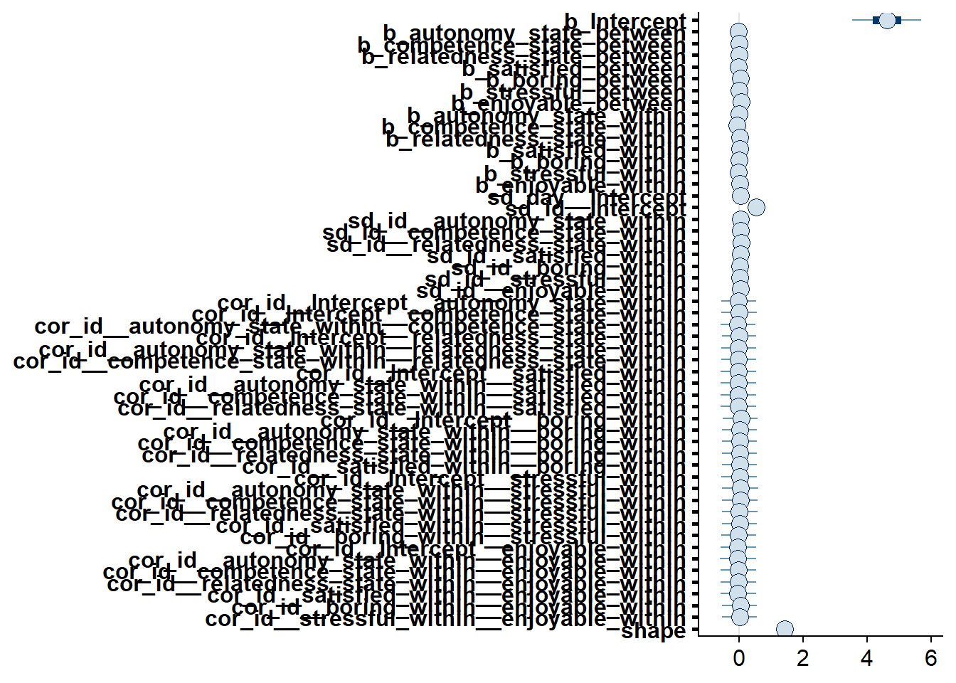

The effects plot (Figure 4.31) visually confirms that none of the predictors seem influential. Note that the correlations between random effects are on different scales which explains why the CI around them are so wide. Except for the correlations, all effects are on the log scale because we used a Gamma distribution, but the correlations are regularly on a scale of -1 to 1.

Figure 4.31: Effects plot for Model 4

4.4.2 Model 5: State variables predicting subjective use

The next model predicts subjective use from the same predictors. Once more, we know that subjective and objective use aren’t perfectly correlated, but the priors for Model 4 again are our best bet here (for both within-person and between-person effects).

priors_model5 <- 
  c(
    # intercept
    prior(normal(4.5, 0.8), class = Intercept),
    
    # prior on effects
    prior(normal(0, 0.1), class = b),
    
    # prior on shape
    prior(gamma(2.5, 100), class = shape)
  )

Let’s run the model. Like with Model 2, we don’t separately model zeros.

model5 <- 
  brm(
    data = dat,
    family = Gamma(link = "log"),
    prior = priors_model4,
    social_media_subjective ~
      1 +
      autonomy_state_between +
      competence_state_between +
      relatedness_state_between +
      satisfied_between +
      boring_between +
      stressful_between +
      enjoyable_between +
      autonomy_state_within +
      competence_state_within +
      relatedness_state_within +
      satisfied_within +
      boring_within +
      stressful_within +
      enjoyable_within +
      (
        1 +
        autonomy_state_within +
        competence_state_within +
        relatedness_state_within +
        satisfied_within +
        boring_within +
        stressful_within +
        enjoyable_within |
        id
      ) +
      (1 |day),
    iter = 5000,
    warmup = 2000,
    chains = 4,
    cores = 4,
    seed = 42,
    control = list(
      adapt_delta = 0.99
    ),
    file = here("models", "model5")
  )

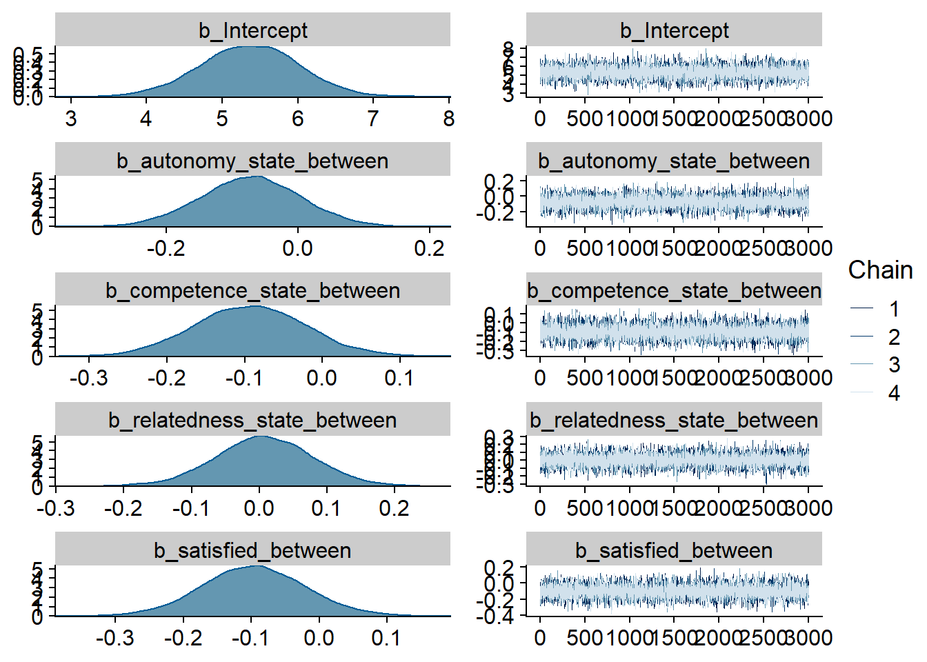
Overall, the traceplots look fine and the chains seem to have mixed well (Figure ??). Like before, the variance around the day grouping is small and mostly estimated to be zero or close to zero.

Figure 4.32: Traceplots and posterior distributions for Model 4

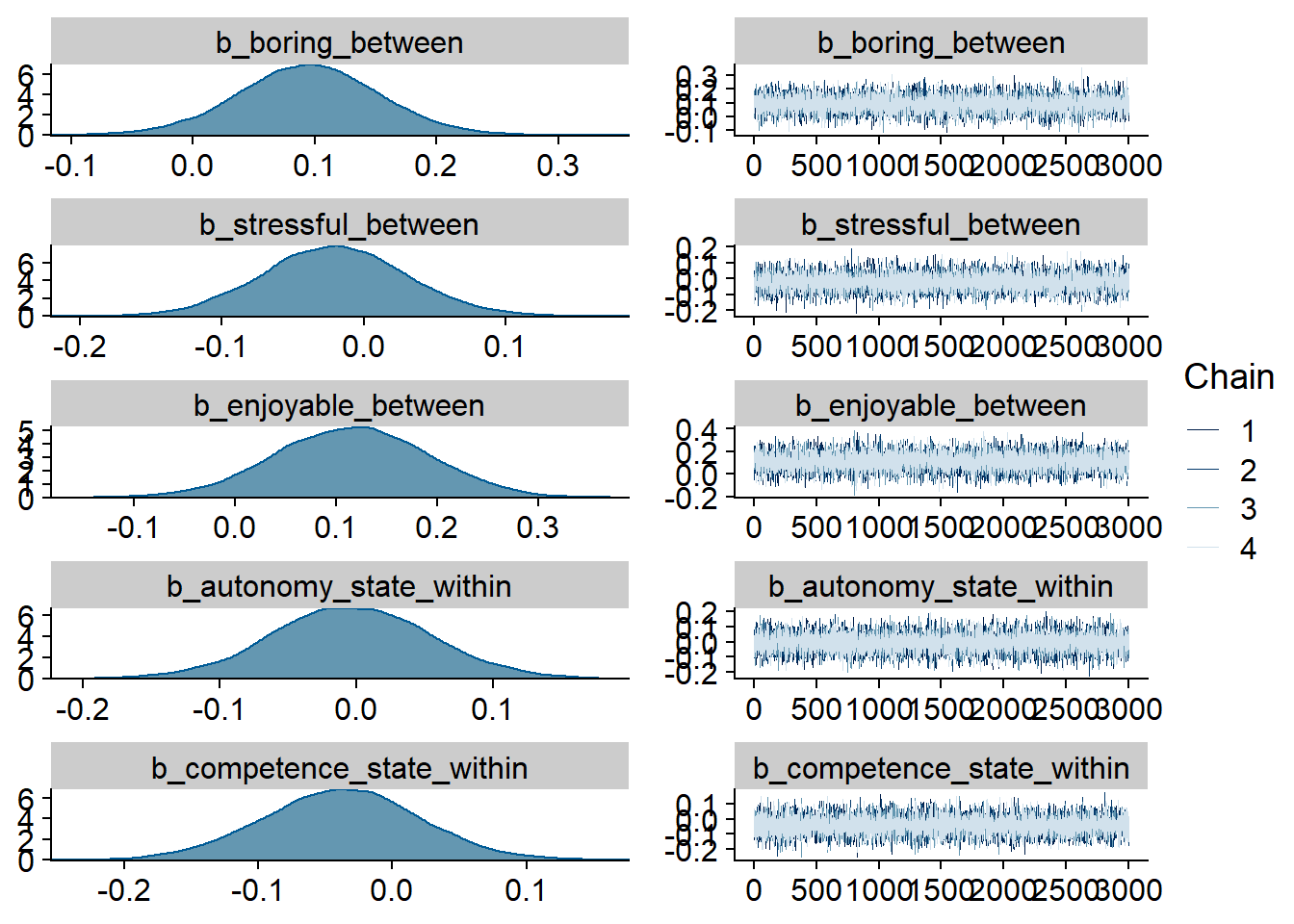
Figure 4.33: Traceplots and posterior distributions for Model 4

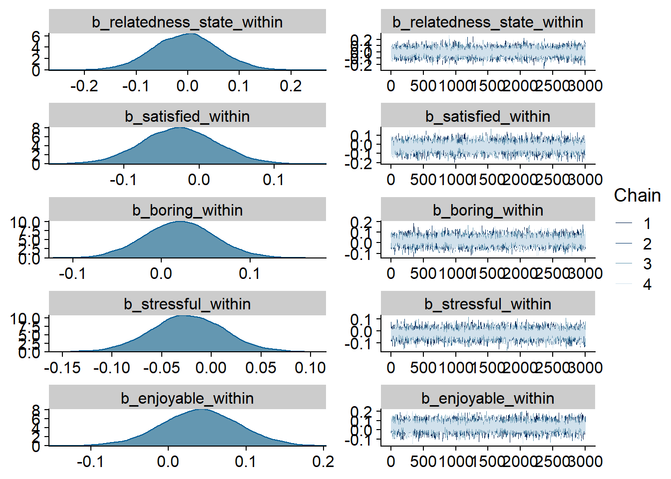
Figure 4.34: Traceplots and posterior distributions for Model 4

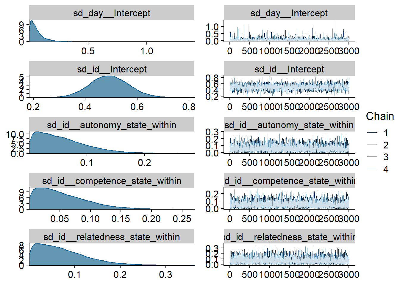
Figure 4.35: Traceplots and posterior distributions for Model 4

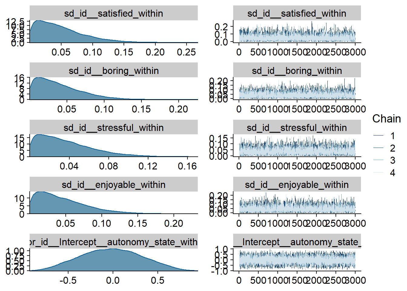
Figure 4.36: Traceplots and posterior distributions for Model 4

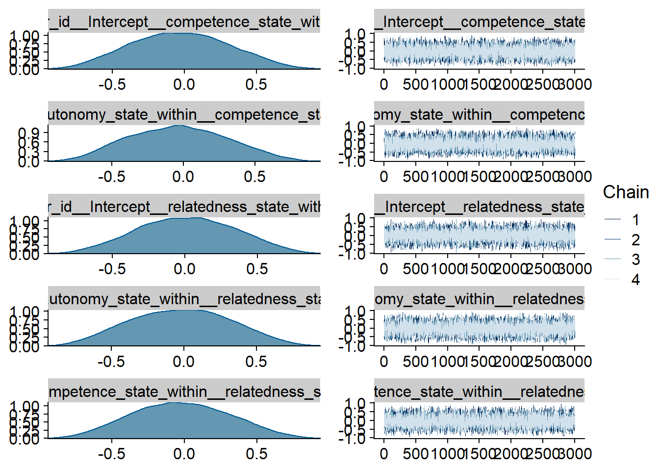
Figure 4.37: Traceplots and posterior distributions for Model 4

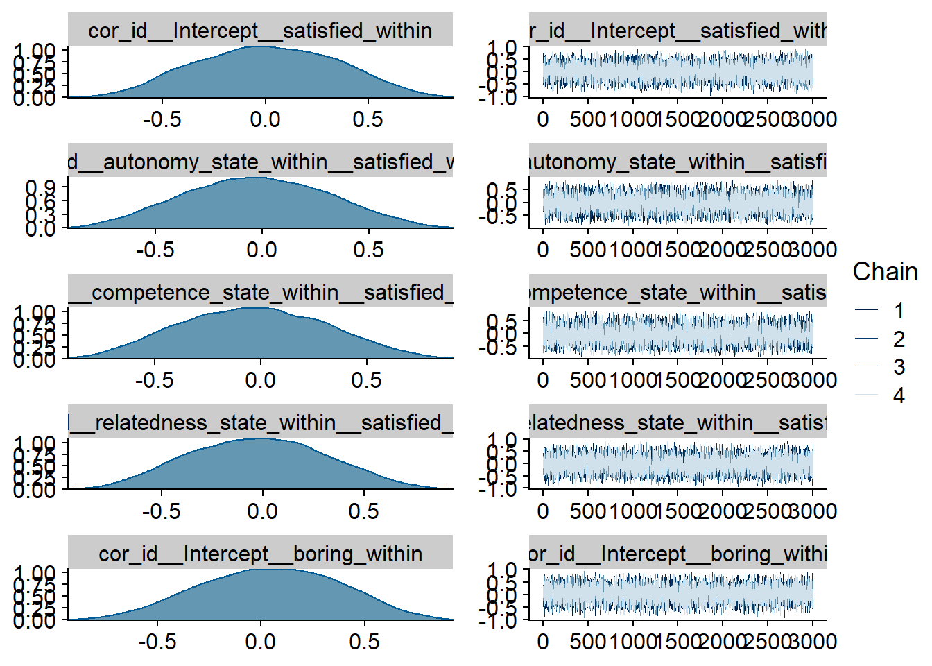
Figure 4.38: Traceplots and posterior distributions for Model 4

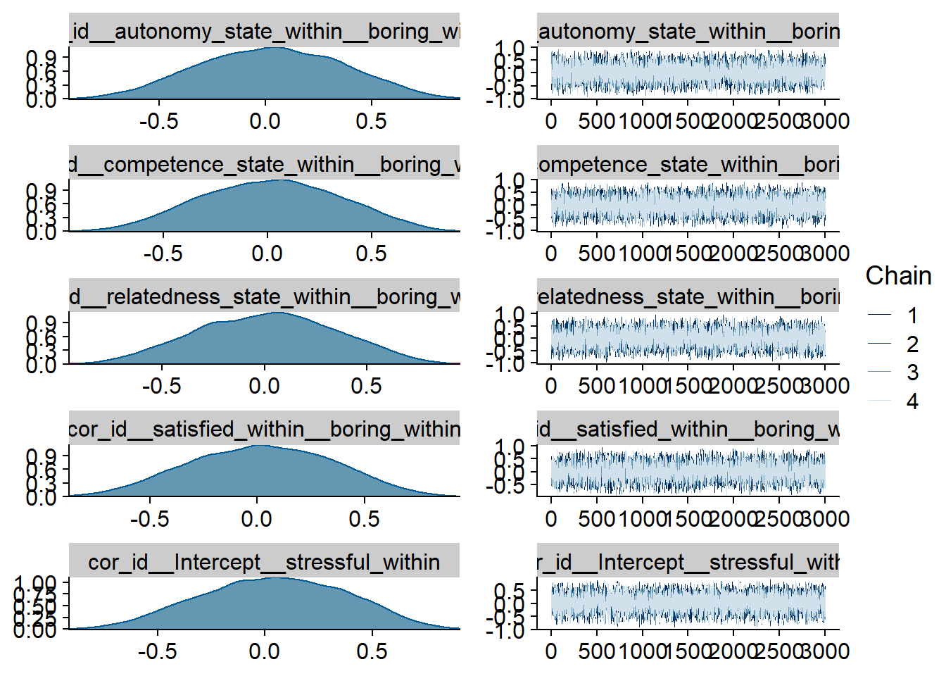
Figure 4.39: Traceplots and posterior distributions for Model 4

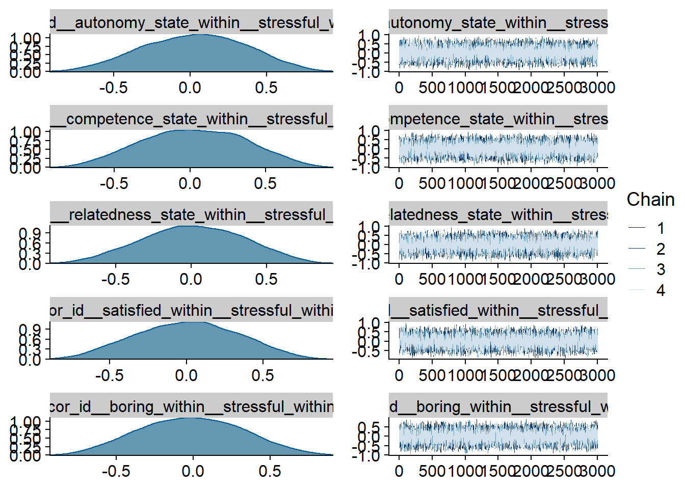
Figure 4.40: Traceplots and posterior distributions for Model 4

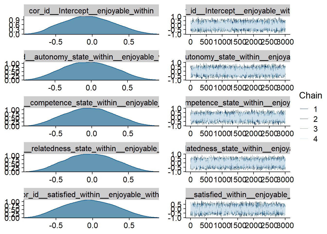
Figure 4.41: Traceplots and posterior distributions for Model 4

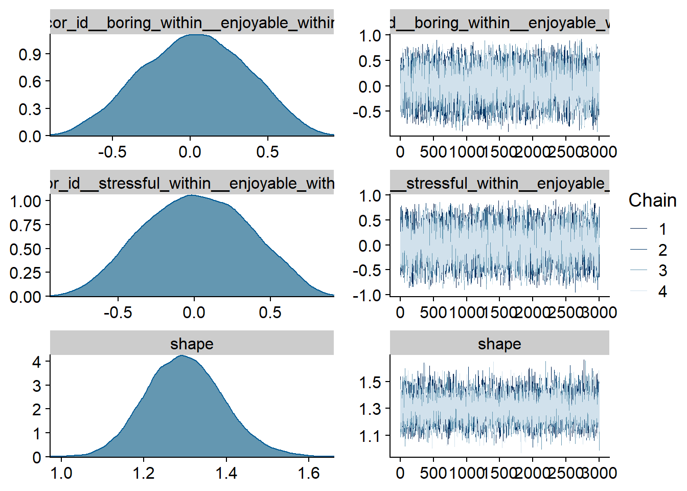
Figure 4.42: Traceplots and posterior distributions for Model 4

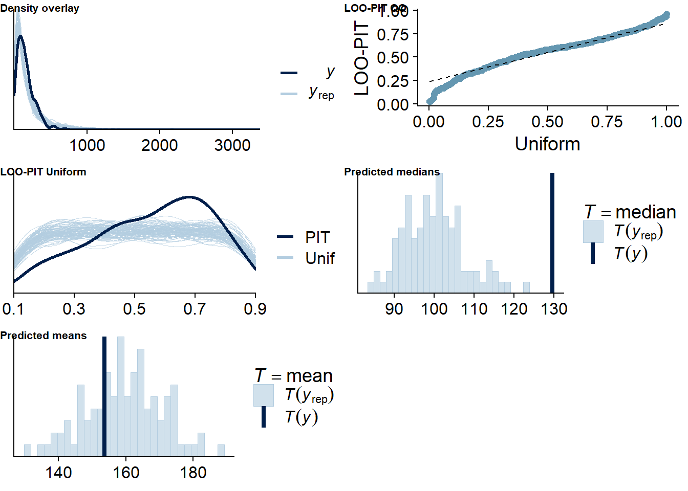
The posterior predictive check shows about the same model fit as Model 4: mediocre. It overestimates the frequency of low values compared to the raw data. I could change the prior, but I also don’t want to overfit just based on the raw data.

Figure 4.43: Posterior predictive checks for Model 5

There are no cases flagged as potentially influential outliers.

loo(model5, reloo = TRUE)

## 1 problematic observation(s) found.
## The model will be refit 1 times.

## 
## Fitting model 1 out of 1 (leaving out observation 384)

## Start sampling

## 
## Computed from 12000 by 420 log-likelihood matrix
## 
##          Estimate   SE
## elpd_loo  -2466.6 15.8
## p_loo        28.8  1.6
## looic      4933.2 31.6
## ------
## Monte Carlo SE of elpd_loo is 0.1.
## 
## Pareto k diagnostic values:
##                          Count Pct.    Min. n_eff
## (-Inf, 0.5]   (good)     393   93.6%   1996      
##  (0.5, 0.7]   (ok)        27    6.4%   1886      
##    (0.7, 1]   (bad)        0    0.0%   <NA>      
##    (1, Inf)   (very bad)   0    0.0%   <NA>      
## 
## All Pareto k estimates are ok (k < 0.7).
## See help('pareto-k-diagnostic') for details.

Let’s inspect the summary. Having an enjoyable and boring day might be related to estimating more social media use (on the between level). Conversely, a feeling of competence might decrease estimates. However, all three of those posterior distributions include zero, even though it’s close.

summary(model5, priors = TRUE)

##  Family: gamma 
##   Links: mu = log; shape = identity 
## Formula: social_media_subjective ~ 1 + autonomy_state_between + competence_state_between + relatedness_state_between + satisfied_between + boring_between + stressful_between + enjoyable_between + autonomy_state_within + competence_state_within + relatedness_state_within + satisfied_within + boring_within + stressful_within + enjoyable_within + (1 + autonomy_state_within + competence_state_within + relatedness_state_within + satisfied_within + boring_within + stressful_within + enjoyable_within | id) + (1 | day) 
##    Data: study1 (Number of observations: 420) 
## Samples: 4 chains, each with iter = 5000; warmup = 2000; thin = 1;
##          total post-warmup samples = 12000
## 
## Priors: 
## b ~ normal(0, 0.1)
## Intercept ~ normal(4.5, 0.8)
## L ~ lkj_corr_cholesky(1)
## sd ~ student_t(3, 0, 2.5)
## shape ~ gamma(2.5, 100)
## 
## Group-Level Effects: 
## ~day (Number of levels: 5) 
##               Estimate Est.Error l-95% CI u-95% CI Rhat Bulk_ESS Tail_ESS
## sd(Intercept)     0.07      0.08     0.00     0.26 1.00     6115     6209
## 
## ~id (Number of levels: 94) 
##                                                       Estimate Est.Error l-95% CI u-95% CI Rhat Bulk_ESS Tail_ESS
## sd(Intercept)                                             0.49      0.08     0.35     0.64 1.00     4609     6905
## sd(autonomy_state_within)                                 0.06      0.04     0.00     0.16 1.00     9124     6247
## sd(competence_state_within)                               0.05      0.04     0.00     0.16 1.00     9417     5712
## sd(relatedness_state_within)                              0.07      0.05     0.00     0.20 1.00    10131     6334
## sd(satisfied_within)                                      0.05      0.04     0.00     0.14 1.00     8222     5408
## sd(boring_within)                                         0.04      0.03     0.00     0.11 1.00     9518     5873
## sd(stressful_within)                                      0.04      0.03     0.00     0.10 1.00     9568     6523
## sd(enjoyable_within)                                      0.04      0.03     0.00     0.13 1.00     8525     6408
## cor(Intercept,autonomy_state_within)                     -0.02      0.34    -0.65     0.63 1.00    26697     8853
## cor(Intercept,competence_state_within)                   -0.03      0.33    -0.65     0.61 1.00    25740     8665
## cor(autonomy_state_within,competence_state_within)       -0.04      0.34    -0.65     0.61 1.00    17150     9376
## cor(Intercept,relatedness_state_within)                   0.01      0.33    -0.63     0.65 1.00    27531     8584
## cor(autonomy_state_within,relatedness_state_within)      -0.02      0.34    -0.66     0.62 1.00    16808     9191
## cor(competence_state_within,relatedness_state_within)    -0.02      0.33    -0.64     0.61 1.00    12371     9241
## cor(Intercept,satisfied_within)                           0.01      0.33    -0.62     0.64 1.00    23477     8466
## cor(autonomy_state_within,satisfied_within)              -0.03      0.33    -0.66     0.62 1.00    16534     8899
## cor(competence_state_within,satisfied_within)            -0.03      0.34    -0.67     0.62 1.00    12832     9212
## cor(relatedness_state_within,satisfied_within)           -0.03      0.33    -0.65     0.61 1.00    10261    10017
## cor(Intercept,boring_within)                              0.04      0.33    -0.60     0.65 1.00    21811     8984
## cor(autonomy_state_within,boring_within)                  0.03      0.33    -0.61     0.66 1.00    17402     9064
## cor(competence_state_within,boring_within)                0.02      0.33    -0.62     0.65 1.00    13863     8855
## cor(relatedness_state_within,boring_within)               0.01      0.34    -0.63     0.64 1.00    10166     9533
## cor(satisfied_within,boring_within)                       0.02      0.33    -0.61     0.64 1.00     9338     9412
## cor(Intercept,stressful_within)                           0.04      0.33    -0.59     0.64 1.00    25952     7970
## cor(autonomy_state_within,stressful_within)               0.03      0.33    -0.62     0.66 1.00    15050     8199
## cor(competence_state_within,stressful_within)             0.03      0.34    -0.62     0.66 1.00    12065     8725
## cor(relatedness_state_within,stressful_within)            0.01      0.33    -0.62     0.64 1.00     9962     9381
## cor(satisfied_within,stressful_within)                    0.01      0.33    -0.62     0.63 1.00     9639     9836
## cor(boring_within,stressful_within)                      -0.01      0.33    -0.64     0.62 1.00     7948     9156
## cor(Intercept,enjoyable_within)                          -0.05      0.33    -0.65     0.59 1.00    24227     9637
## cor(autonomy_state_within,enjoyable_within)              -0.03      0.34    -0.66     0.61 1.00    15460     8292
## cor(competence_state_within,enjoyable_within)            -0.03      0.33    -0.65     0.60 1.00    12580     8950
## cor(relatedness_state_within,enjoyable_within)           -0.02      0.33    -0.64     0.61 1.00    11135     9699
## cor(satisfied_within,enjoyable_within)                   -0.04      0.34    -0.67     0.60 1.00     8582     9049
## cor(boring_within,enjoyable_within)                       0.03      0.33    -0.62     0.65 1.00     8034     9232
## cor(stressful_within,enjoyable_within)                    0.02      0.34    -0.63     0.66 1.00     6775    10061
## 
## Population-Level Effects: 
##                           Estimate Est.Error l-95% CI u-95% CI Rhat Bulk_ESS Tail_ESS
## Intercept                     5.36      0.66     4.06     6.63 1.00    11737    10046
## autonomy_state_between       -0.07      0.08    -0.22     0.08 1.00    13941     8408
## competence_state_between     -0.09      0.07    -0.23     0.05 1.00    12371     9819
## relatedness_state_between     0.01      0.07    -0.14     0.15 1.00    14157     8970
## satisfied_between            -0.10      0.08    -0.25     0.05 1.00    13708     8537
## boring_between                0.09      0.06    -0.02     0.21 1.00    11432     9251
## stressful_between            -0.02      0.05    -0.12     0.08 1.00    10961     9963
## enjoyable_between             0.12      0.08    -0.03     0.26 1.00    13528     9775
## autonomy_state_within        -0.00      0.06    -0.12     0.11 1.00    23098     9607
## competence_state_within      -0.04      0.06    -0.15     0.07 1.00    19223     8865
## relatedness_state_within     -0.00      0.06    -0.13     0.12 1.00    23114     9482
## satisfied_within             -0.03      0.05    -0.12     0.07 1.00    18050     9322
## boring_within                 0.02      0.04    -0.06     0.10 1.00    21043     9152
## stressful_within             -0.02      0.04    -0.10     0.05 1.00    22686     9812
## enjoyable_within              0.04      0.05    -0.06     0.14 1.00    19642     8730
## 
## Family Specific Parameters: 
##       Estimate Est.Error l-95% CI u-95% CI Rhat Bulk_ESS Tail_ESS
## shape     1.30      0.09     1.12     1.49 1.00    11230     9042
## 
## Samples were drawn using sampling(NUTS). For each parameter, Bulk_ESS
## and Tail_ESS are effective sample size measures, and Rhat is the potential
## scale reduction factor on split chains (at convergence, Rhat = 1).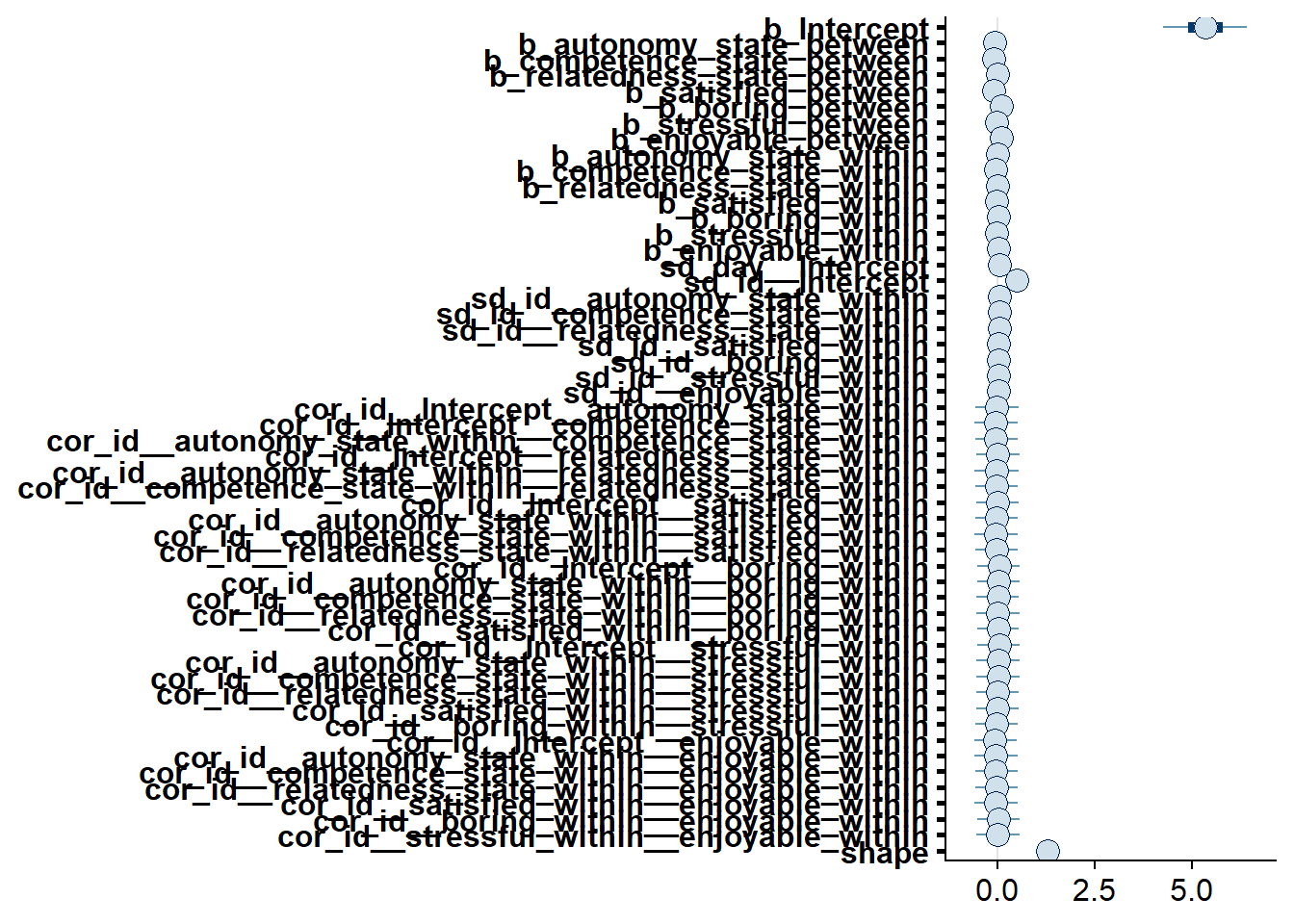

The effects plot (Figure 4.44) visually that those three states might be influential, but their CIs overlap with zero.

Figure 4.44: Effects plot for Model 5

4.4.3 Model 6: State variables predicting accuracy

For this model, once more it’s hard to choose informed priors. Therefore, I choose the same skeptical, but weakly regularizing priors as for Model 3, with a student t distribution with fat tails, an intercept that reflects a tendency to overestimate, and slopes that are skeptical of large effects. For everything else, I’ll use the brms default priors because I don’t have information on what correlation or variances to expect. Note that I use the priors on the slope for both between and within effects, simply because I don’t have an informed guess about the two being different.

priors_model6 <- 
  c(
    # intercept
    prior(student_t(10, 20, 100), class = Intercept),
    
    # all other effects
    prior(normal(0, 25), class = b)
  )

Let’s run the model.

model6 <- 
  brm(
    data = dat,
    family = student,
    prior = priors_model6,
    error ~
      1 +
      autonomy_state_between +
      competence_state_between +
      relatedness_state_between +
      satisfied_between +
      boring_between +
      stressful_between +
      enjoyable_between +
      autonomy_state_within +
      competence_state_within +
      relatedness_state_within +
      satisfied_within +
      boring_within +
      stressful_within +
      enjoyable_within +
      (
        1 +
        autonomy_state_within +
        competence_state_within +
        relatedness_state_within +
        satisfied_within +
        boring_within +
        stressful_within +
        enjoyable_within |
        id
      ) +
      (1 |day),
    iter = 5000,
    warmup = 2000,
    chains = 4,
    cores = 4,
    seed = 42,
    control = list(
      adapt_delta = 0.99
    ),
    file = here("models", "model6")
  )

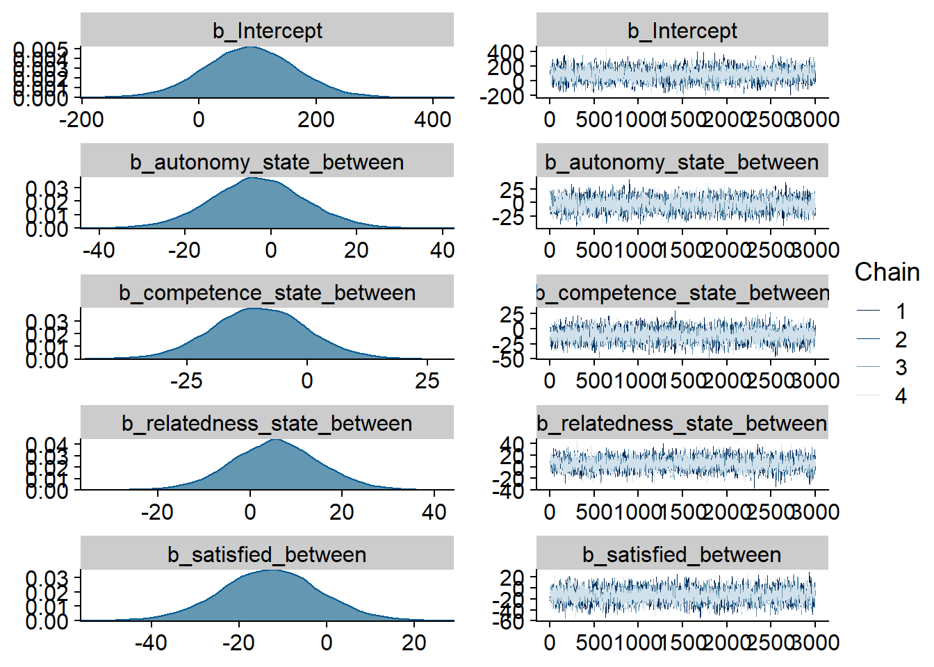
Overall, the traceplots look fine and the chains seem to have mixed well, see (Figure ??), just like with Model 3.

Figure 4.45: Traceplots and posterior distributions for Model 6

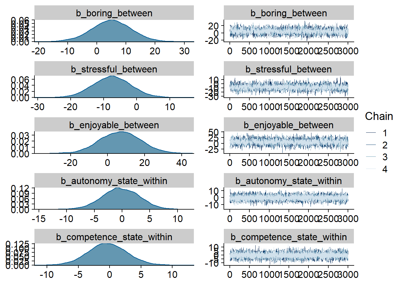
Figure 4.46: Traceplots and posterior distributions for Model 6

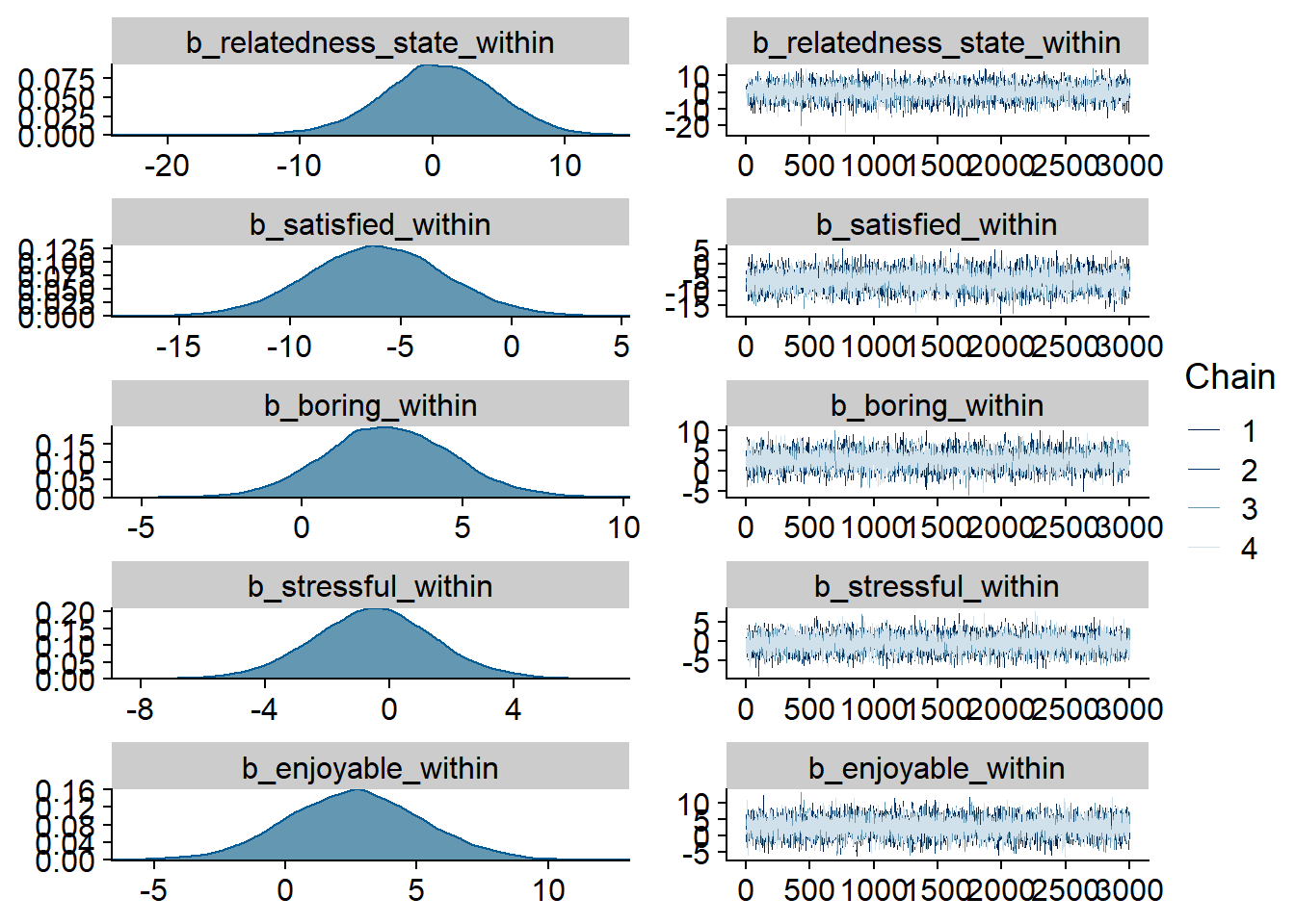
Figure 4.47: Traceplots and posterior distributions for Model 6

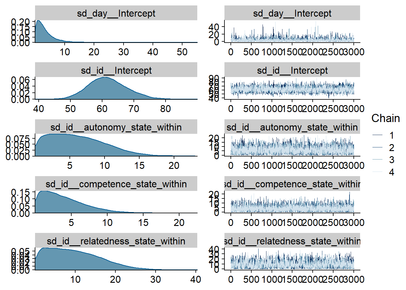
Figure 4.48: Traceplots and posterior distributions for Model 6

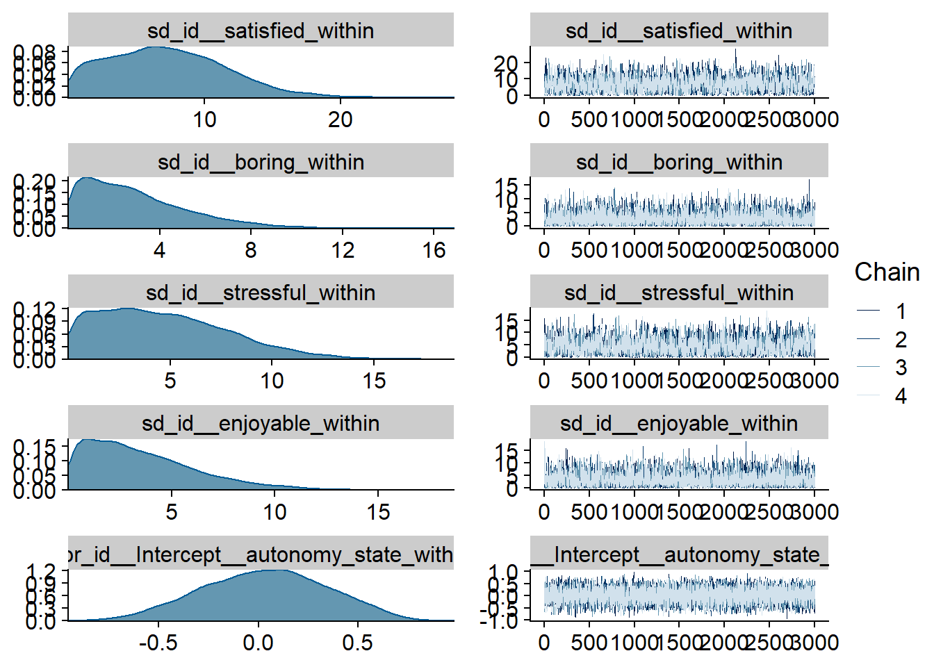
Figure 4.49: Traceplots and posterior distributions for Model 6

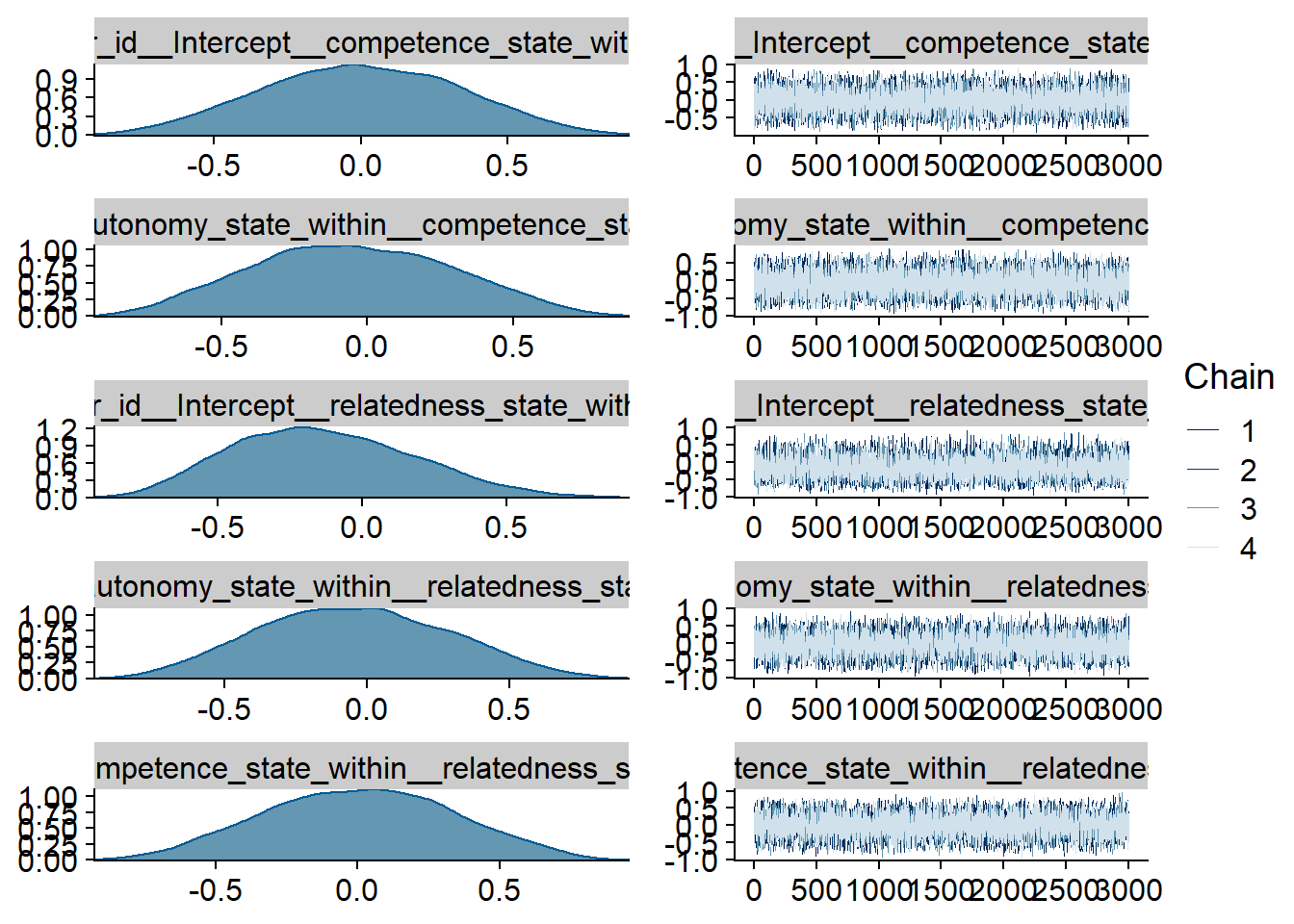
Figure 4.50: Traceplots and posterior distributions for Model 6

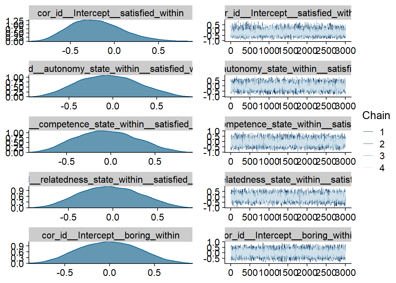
Figure 4.51: Traceplots and posterior distributions for Model 6

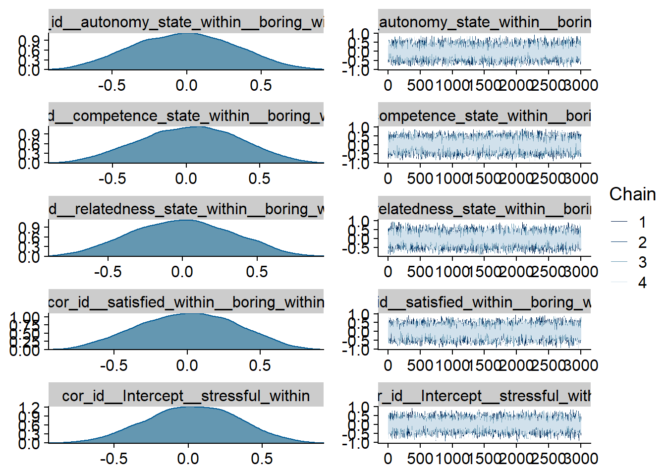
Figure 4.52: Traceplots and posterior distributions for Model 6

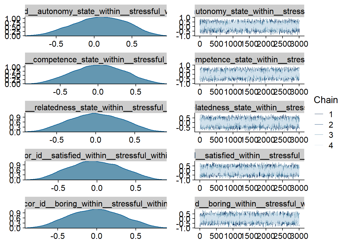
Figure 4.53: Traceplots and posterior distributions for Model 6

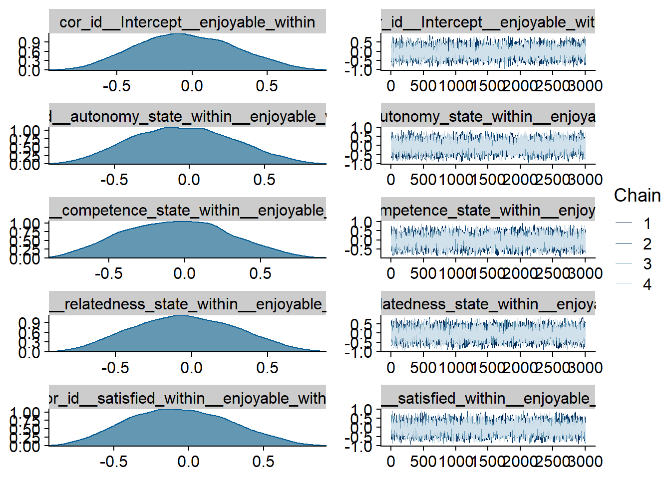
Figure 4.54: Traceplots and posterior distributions for Model 6

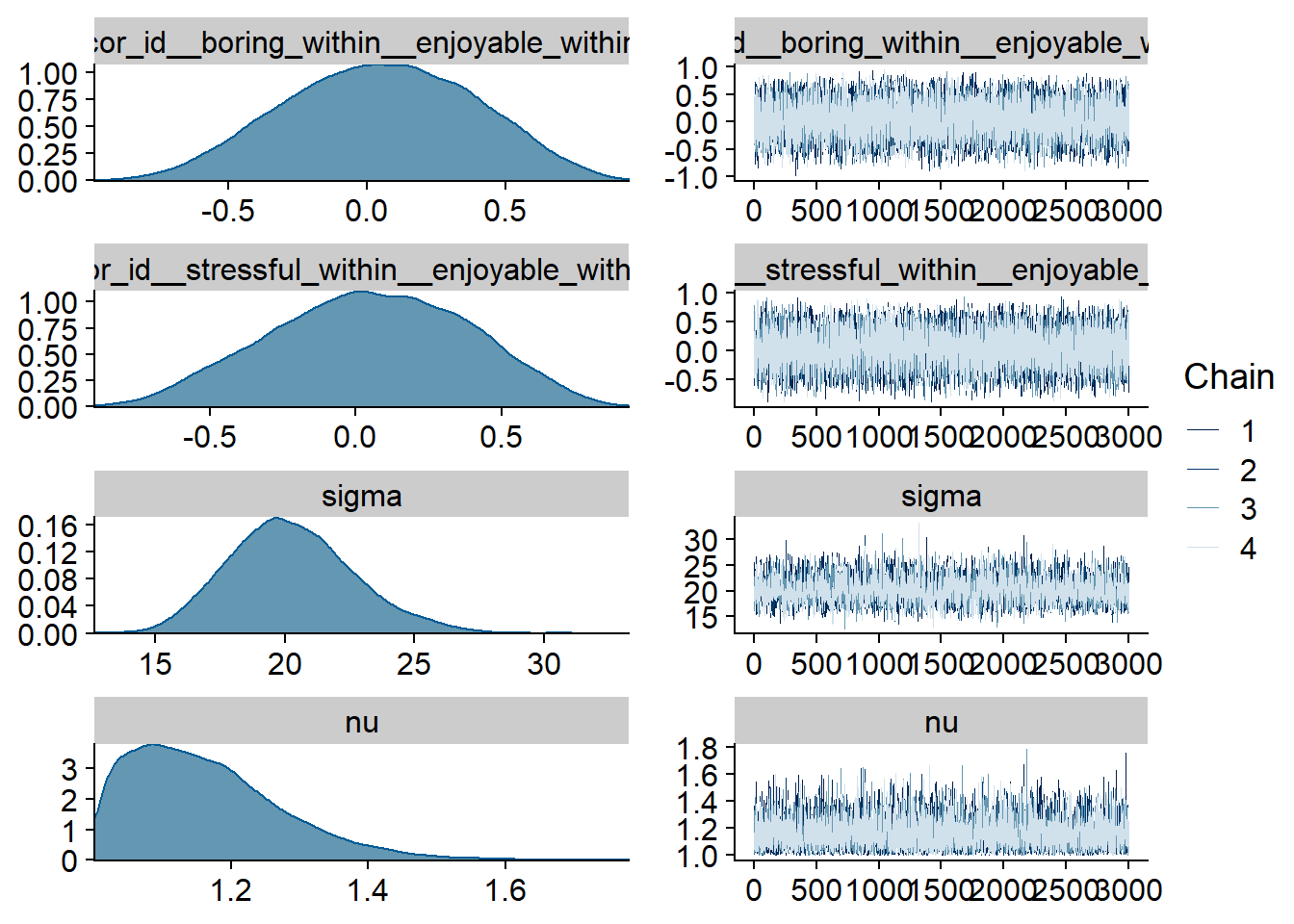
Figure 4.55: Traceplots and posterior distributions for Model 6

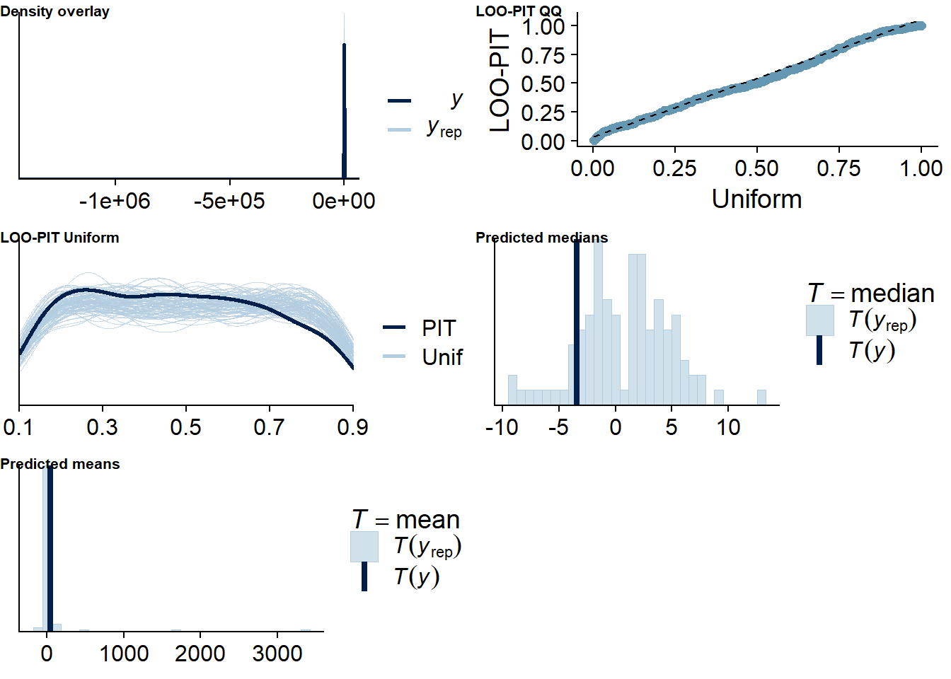
The posterior predictive checks (Figure ??) look good. Like with Model 3, that the upper left panel looks strange because of the massive scale on the x-axis. I reproduce it again at the bottom with a more sensible x-axis. Once more, the student t distribution assigns too much posterior mass to negative values, whereas the data are right skewed. Otherwise, the model does an okay job in recovering the mean and the median.

Figure 4.56: Posterior predictive checks for Model 6

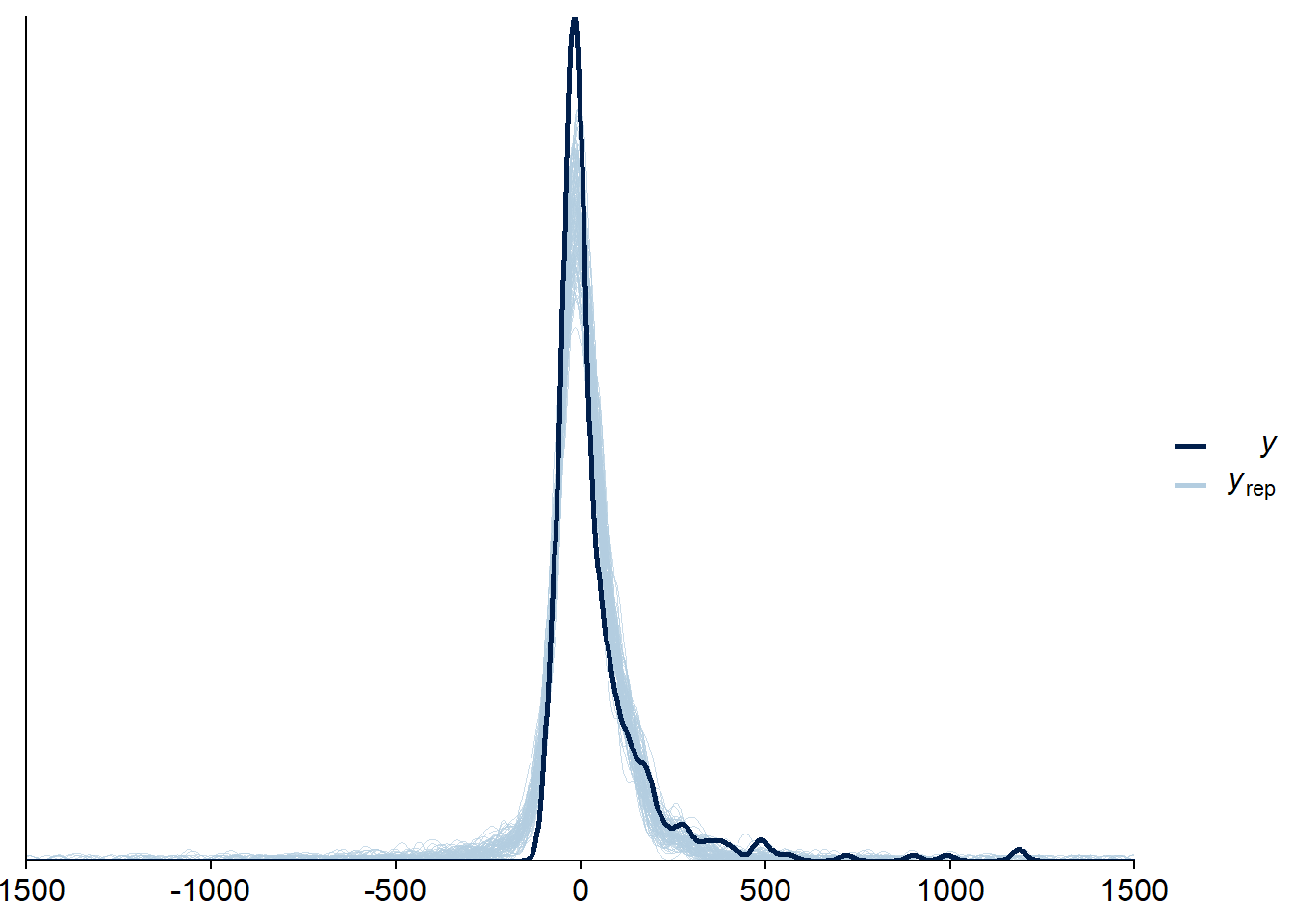
Figure 4.57: Posterior predictive checks for Model 6

Two cases are flagged as potential outliers, which disappear once calculated directly.

loo(model6, reloo = TRUE)

## 2 problematic observation(s) found.
## The model will be refit 2 times.

## 
## Fitting model 1 out of 2 (leaving out observation 39)

## 
## Fitting model 2 out of 2 (leaving out observation 128)

## Start sampling
## Start sampling

## 
## Computed from 12000 by 418 log-likelihood matrix
## 
##          Estimate   SE
## elpd_loo  -2368.1 30.7
## p_loo       204.2  7.8
## looic      4736.3 61.4
## ------
## Monte Carlo SE of elpd_loo is 0.2.
## 
## Pareto k diagnostic values:
##                          Count Pct.    Min. n_eff
## (-Inf, 0.5]   (good)     415   99.3%   524       
##  (0.5, 0.7]   (ok)         3    0.7%   965       
##    (0.7, 1]   (bad)        0    0.0%   <NA>      
##    (1, Inf)   (very bad)   0    0.0%   <NA>      
## 
## All Pareto k estimates are ok (k < 0.7).
## See help('pareto-k-diagnostic') for details.

Let’s inspect the summary. All posteriors include 0, only satisfaction (within) comes close.

summary(model6, priors = TRUE)

##  Family: student 
##   Links: mu = identity; sigma = identity; nu = identity 
## Formula: error ~ 1 + autonomy_state_between + competence_state_between + relatedness_state_between + satisfied_between + boring_between + stressful_between + enjoyable_between + autonomy_state_within + competence_state_within + relatedness_state_within + satisfied_within + boring_within + stressful_within + enjoyable_within + (1 + autonomy_state_within + competence_state_within + relatedness_state_within + satisfied_within + boring_within + stressful_within + enjoyable_within | id) + (1 | day) 
##    Data: study1 (Number of observations: 418) 
## Samples: 4 chains, each with iter = 5000; warmup = 2000; thin = 1;
##          total post-warmup samples = 12000
## 
## Priors: 
## b ~ normal(0, 25)
## Intercept ~ student_t(10, 20, 100)
## L ~ lkj_corr_cholesky(1)
## nu ~ gamma(2, 0.1)
## sd ~ student_t(3, 0, 56.4)
## sigma ~ student_t(3, 0, 56.4)
## 
## Group-Level Effects: 
## ~day (Number of levels: 5) 
##               Estimate Est.Error l-95% CI u-95% CI Rhat Bulk_ESS Tail_ESS
## sd(Intercept)     3.42      3.53     0.12    12.17 1.00     7456     7118
## 
## ~id (Number of levels: 94) 
##                                                       Estimate Est.Error l-95% CI u-95% CI Rhat Bulk_ESS Tail_ESS
## sd(Intercept)                                            61.71      6.13    50.50    74.40 1.00     2533     5226
## sd(autonomy_state_within)                                 6.08      3.99     0.35    14.85 1.00     3444     5438
## sd(competence_state_within)                               3.93      2.98     0.16    11.07 1.00     5720     6710
## sd(relatedness_state_within)                              9.65      6.50     0.45    23.82 1.00     1877     3608
## sd(satisfied_within)                                      7.20      4.24     0.43    16.23 1.00     2343     4739
## sd(boring_within)                                         2.93      2.28     0.10     8.42 1.00     4427     5807
## sd(stressful_within)                                      4.68      3.13     0.21    11.56 1.00     1907     4368
## sd(enjoyable_within)                                      3.54      2.65     0.15     9.98 1.00     4206     6088
## cor(Intercept,autonomy_state_within)                      0.03      0.31    -0.57     0.61 1.00    11743     8439
## cor(Intercept,competence_state_within)                    0.00      0.33    -0.63     0.64 1.00    15909     8803
## cor(autonomy_state_within,competence_state_within)       -0.05      0.34    -0.68     0.60 1.00    12817     9811
## cor(Intercept,relatedness_state_within)                  -0.14      0.31    -0.68     0.51 1.00     7624     8454
## cor(autonomy_state_within,relatedness_state_within)      -0.05      0.33    -0.66     0.60 1.00     7309     8183
## cor(competence_state_within,relatedness_state_within)     0.00      0.33    -0.62     0.63 1.00     7938     9181
## cor(Intercept,satisfied_within)                          -0.20      0.30    -0.71     0.44 1.00     9855     8185
## cor(autonomy_state_within,satisfied_within)              -0.05      0.33    -0.67     0.61 1.00     6581     8107
## cor(competence_state_within,satisfied_within)            -0.05      0.33    -0.66     0.61 1.00     6539     8703
## cor(relatedness_state_within,satisfied_within)           -0.03      0.33    -0.64     0.61 1.00     7108     8023
## cor(Intercept,boring_within)                             -0.01      0.33    -0.62     0.62 1.00    15554     9548
## cor(autonomy_state_within,boring_within)                 -0.01      0.33    -0.64     0.62 1.00    12145     9704
## cor(competence_state_within,boring_within)                0.02      0.33    -0.61     0.64 1.00    10078     9187
## cor(relatedness_state_within,boring_within)              -0.00      0.33    -0.63     0.63 1.00    11403    10241
## cor(satisfied_within,boring_within)                       0.01      0.33    -0.63     0.63 1.00    11135    10441
## cor(Intercept,stressful_within)                           0.03      0.30    -0.56     0.60 1.00    12347     8296
## cor(autonomy_state_within,stressful_within)               0.08      0.34    -0.58     0.69 1.00     6490     7890
## cor(competence_state_within,stressful_within)             0.01      0.33    -0.63     0.64 1.00     6964     8863
## cor(relatedness_state_within,stressful_within)            0.00      0.33    -0.62     0.62 1.00     7347     9079
## cor(satisfied_within,stressful_within)                   -0.02      0.33    -0.63     0.60 1.00     6808     9360
## cor(boring_within,stressful_within)                      -0.01      0.33    -0.62     0.62 1.00     7663     9685
## cor(Intercept,enjoyable_within)                          -0.04      0.32    -0.63     0.59 1.00    16828     8556
## cor(autonomy_state_within,enjoyable_within)              -0.04      0.33    -0.66     0.61 1.00    12316     9356
## cor(competence_state_within,enjoyable_within)            -0.05      0.34    -0.69     0.61 1.00    10687     9355
## cor(relatedness_state_within,enjoyable_within)           -0.04      0.33    -0.66     0.60 1.00     9867     9262
## cor(satisfied_within,enjoyable_within)                   -0.06      0.33    -0.67     0.60 1.00    10953    10778
## cor(boring_within,enjoyable_within)                       0.05      0.34    -0.60     0.68 1.00     9391    10550
## cor(stressful_within,enjoyable_within)                    0.05      0.33    -0.60     0.66 1.00     8960     9976
## 
## Population-Level Effects: 
##                           Estimate Est.Error l-95% CI u-95% CI Rhat Bulk_ESS Tail_ESS
## Intercept                    86.88     77.56   -65.70   238.81 1.00     2752     4530
## autonomy_state_between       -3.04     11.00   -24.81    18.66 1.00     3174     5822
## competence_state_between     -9.97      9.92   -29.55     9.69 1.00     3299     5130
## relatedness_state_between     5.55      9.55   -13.26    24.35 1.00     3147     5114
## satisfied_between           -13.00     11.32   -35.48     9.26 1.00     2544     4848
## boring_between                4.97      6.81    -8.76    18.30 1.00     2619     4431
## stressful_between            -7.55      5.83   -18.90     3.92 1.00     3106     5140
## enjoyable_between             6.88     11.12   -14.52    28.89 1.00     2708     5134
## autonomy_state_within        -0.25      3.34    -6.83     6.22 1.00    11063     9397
## competence_state_within      -0.35      3.15    -6.57     5.92 1.00    10688     8919
## relatedness_state_within      0.48      4.28    -8.21     8.64 1.00     7366     8089
## satisfied_within             -6.06      3.09   -12.11     0.06 1.00     9937     9359
## boring_within                 2.70      2.01    -1.17     6.75 1.00     9306     9585
## stressful_within             -0.49      1.95    -4.34     3.40 1.00    10024     9298
## enjoyable_within              2.63      2.57    -2.37     7.69 1.00     9981     9549
## 
## Family Specific Parameters: 
##       Estimate Est.Error l-95% CI u-95% CI Rhat Bulk_ESS Tail_ESS
## sigma    20.25      2.41    15.96    25.44 1.00     3054     5285
## nu        1.16      0.11     1.01     1.42 1.00     6060     6060
## 
## Samples were drawn using sampling(NUTS). For each parameter, Bulk_ESS
## and Tail_ESS are effective sample size measures, and Rhat is the potential
## scale reduction factor on split chains (at convergence, Rhat = 1).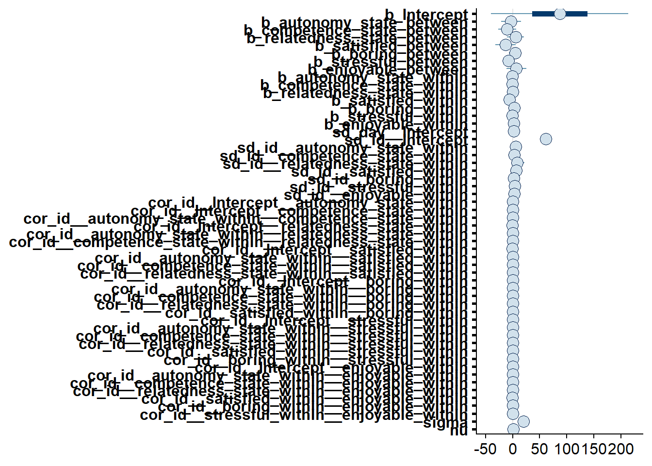

The effects plot (Figure 4.58) visually confirms what I wrote above. Note the difference in scale: everything except the correlations are in percent error, whereas the correlations are on their -1 to 1 scale.

Figure 4.58: Effects plot for Model 6

4.5 Does social media use predict well-being?

For this RQ, we have three questions blocks. We want to know how day-level social media use (both types) and accuracy are related to well-being.

The three questions are: 1. Does objective-only engagement predict day-level well-being? 2. Does subjective-only engagement predict day-level well-being? 3. Does accuracy predict day-level well-being?

4.5.1 Model 7: Objective use predicting well-being

For this model, we’ll predict well-being on that day with objective social media use on that day. Priors here can be controversial, depending on what literature we look to. Well-being is often left-skewed, so we could go for a skewed normal distribution for the model. However, that might be too strong an assumption, which is why I’ll use a model that assumes a normal Gaussian distribution.

As for the specific priors:

When social media use is at zero between people and at zero within, I’ll simply assume a normal distribution centered on the midpoint of the scale (i.e., 3). As for the SD of that distribution, we know the bounds of the scale, so an SD of 1 will have 95% of cases within 1 and 5, which is exactly what we want.
As for the slopes: There are two papers I know of that found a negative, small effect, but another paper that found a negligent one. The larger literature on self-reported media use and well-being also finds very small negative effects, in the range of \(\beta\) = .05. We’re on the unstandardized scale here. So if we assume that well-being is at the midpoint of the scale (i.e., 3), the maximum effect an increase in social media time could have is to bring well-being to its ceiling or floor. That would imply a standard deviation of 1 again - that depends on the scale of the predictor, though. Right now, it’s in minutes and we’d need to scale the prior accordingly. This paper found that with each increase of one standard deviation in social media time, well-being on a 7-point Likert-scale went down by -.06 units. The standard deviation was 190. Therefore (with some crude math), one hour of social media use was associated with 190/60 * -.06 = -0.19 raw units on the outcome scale. From the literature we also know that massive (unstandardized) effects are rare if impossible. Therefore, I’ll center the slope distribution on a small negative value. To be conservative, I’ll take about 75% of the -.19 we found above (say -0.15 Likert-scales) with a somewhat tight standard deviation (say 0.3). This way, 95% of effects will be within -.75 (-.15 + (2 times 0.2)) and 0.45 Likert-points on the outcome scale. Note that we’re on the between-level here: a user with one more hour of social media use will report, on average, a .15 lower score on well-being than someone else with an hour less.
As for the within-effect, most research points toward negligible within-effects, and all of them are on self-reported media use. So here I’ll assume a slopes that varies around zero, but I’ll allow a wider standard deviation than for the between-effect, 0.4. That way, the average within-person effect will be zero and it assumes that 95% of effects are within -0.8 and + 0.8 Likert-points.
For everything else, I’ll once more go with the default brms priors.

Let’s set those priors. Note that we’re still on the minute scale for the predictor, but I specified priors above for hours. That’s why I transform the social media variables to hours (and center) to make interpretation easier. That also helps us set the priors we specified above.

# create hour variables
dat <- 
  dat %>% 
  mutate(
    across(
      c(social_media_objective, social_media_subjective),
      ~ .x / 60, #  divide by 60 to get hours
      .names = "{col}_hours"
    )
  )

# center to get between and within variables
dat <- 
  dat %>% 
  group_by(id) %>% 
  mutate(
    across(
      ends_with("hours"),
      list(
        between = ~ mean(.x, na.rm = TRUE),
        within = ~.x - mean(.x, na.rm = TRUE)
      )
    )
  ) %>% 
  ungroup()

# set priors
priors_model7 <- 
  c(
    # intercept
    prior(normal(3, 1), class = Intercept),
    
    # slopes for between
    prior(normal(-0.15, 0.30), class = b, coef = "social_media_objective_hours_between"),
    
    # slopes for between
    prior(normal(0, 0.40), class = b, coef = "social_media_objective_hours_within")
  )

Okay, let’s run the model.

model7 <- 
  brm(
    data = dat,
    family = gaussian,
    prior = priors_model7,
    well_being_state ~
      1 +
      social_media_objective_hours_between +
      social_media_objective_hours_within +
      (
        1 +
        social_media_objective_hours_within |
        id
      ) +
      (1 |day),
    iter = 5000,
    warmup = 2000,
    chains = 4,
    cores = 4,
    seed = 42,
    control = list(
      adapt_delta = 0.99
    ),
    file = here("models", "model7")
  )

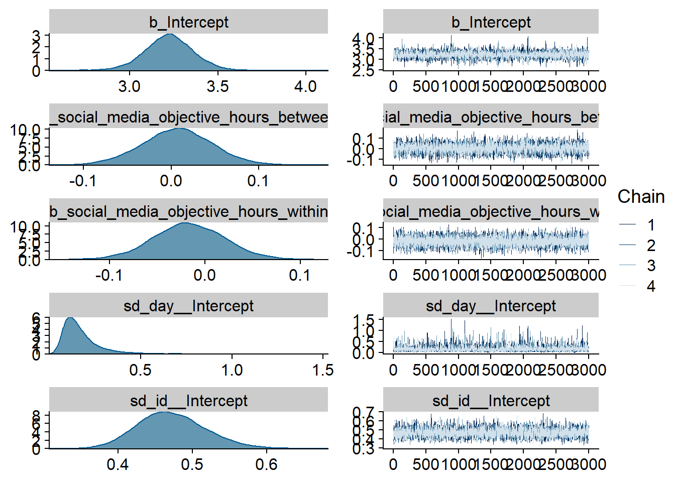
Overall, the traceplots look fine and the chains seem to have mixed well, see (Figure ??).

Figure 4.59: Traceplots and posterior distributions for Model 7

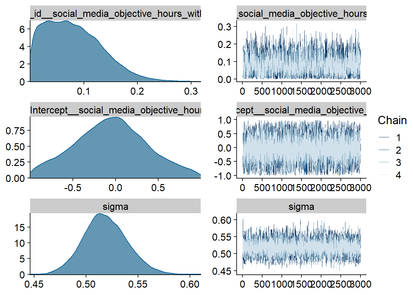
Figure 4.60: Traceplots and posterior distributions for Model 7

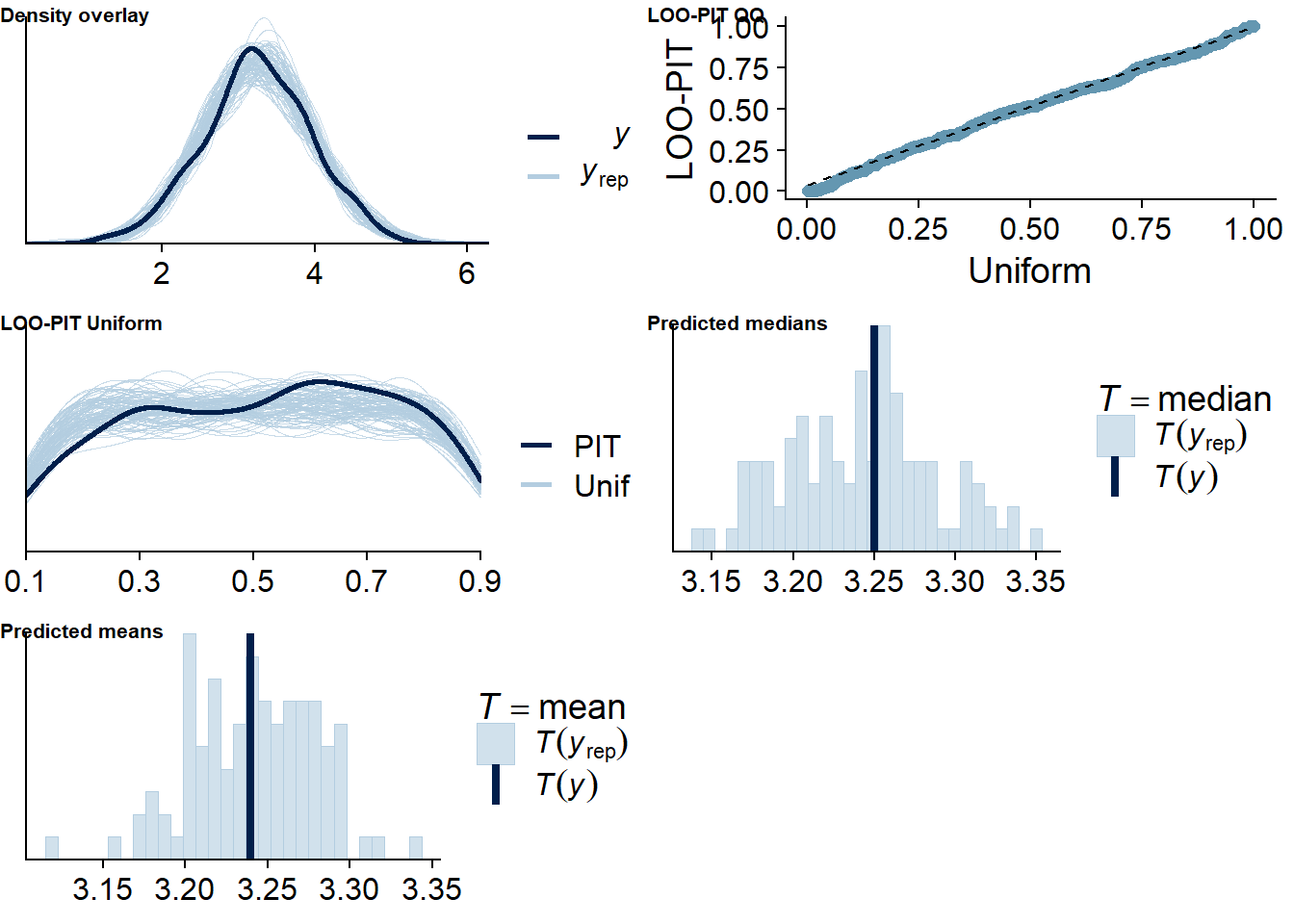
The posterior predictive checks (Figure 4.61) look excellent (no surprise with only one predictor).

Figure 4.61: Posterior predictive checks for Model 7

One case is flagged as potentially influential, but unproblematic when calculated directly.

loo(model7, reloo = TRUE)

## 1 problematic observation(s) found.
## The model will be refit 1 times.

## 
## Fitting model 1 out of 1 (leaving out observation 65)

## Start sampling

## 
## Computed from 12000 by 425 log-likelihood matrix
## 
##          Estimate   SE
## elpd_loo   -370.4 16.1
## p_loo        79.0  5.3
## looic       740.7 32.2
## ------
## Monte Carlo SE of elpd_loo is 0.1.
## 
## Pareto k diagnostic values:
##                          Count Pct.    Min. n_eff
## (-Inf, 0.5]   (good)     410   96.5%   1038      
##  (0.5, 0.7]   (ok)        15    3.5%   569       
##    (0.7, 1]   (bad)        0    0.0%   <NA>      
##    (1, Inf)   (very bad)   0    0.0%   <NA>      
## 
## All Pareto k estimates are ok (k < 0.7).
## See help('pareto-k-diagnostic') for details.

Let’s inspect the summary. The relation is estimated to be extremely close to zero, so really no interpretative wiggle room there. I think this is pretty convincing evidence for the lack of an effect.

summary(model7, priors = TRUE)

##  Family: gaussian 
##   Links: mu = identity; sigma = identity 
## Formula: well_being_state ~ 1 + social_media_objective_hours_between + social_media_objective_hours_within + (1 + social_media_objective_hours_within | id) + (1 | day) 
##    Data: study1 (Number of observations: 425) 
## Samples: 4 chains, each with iter = 5000; warmup = 2000; thin = 1;
##          total post-warmup samples = 12000
## 
## Priors: 
## b_social_media_objective_hours_between ~ normal(-0.15, 0.3)
## b_social_media_objective_hours_within ~ normal(0, 0.4)
## Intercept ~ normal(3, 1)
## L ~ lkj_corr_cholesky(1)
## sd ~ student_t(3, 0, 2.5)
## sigma ~ student_t(3, 0, 2.5)
## 
## Group-Level Effects: 
## ~day (Number of levels: 5) 
##               Estimate Est.Error l-95% CI u-95% CI Rhat Bulk_ESS Tail_ESS
## sd(Intercept)     0.17      0.11     0.05     0.47 1.00     3575     5449
## 
## ~id (Number of levels: 94) 
##                                                    Estimate Est.Error l-95% CI u-95% CI Rhat Bulk_ESS Tail_ESS
## sd(Intercept)                                          0.47      0.05     0.39     0.57 1.00     4536     7237
## sd(social_media_objective_hours_within)                0.08      0.05     0.00     0.20 1.00     3112     4958
## cor(Intercept,social_media_objective_hours_within)    -0.05      0.42    -0.86     0.80 1.00    10858     6678
## 
## Population-Level Effects: 
##                                      Estimate Est.Error l-95% CI u-95% CI Rhat Bulk_ESS Tail_ESS
## Intercept                                3.22      0.14     2.94     3.50 1.00     4255     5282
## social_media_objective_hours_between     0.01      0.04    -0.07     0.08 1.00     5089     6626
## social_media_objective_hours_within     -0.02      0.04    -0.09     0.06 1.00    15746     8839
## 
## Family Specific Parameters: 
##       Estimate Est.Error l-95% CI u-95% CI Rhat Bulk_ESS Tail_ESS
## sigma     0.52      0.02     0.48     0.56 1.00    10146     8819
## 
## Samples were drawn using sampling(NUTS). For each parameter, Bulk_ESS
## and Tail_ESS are effective sample size measures, and Rhat is the potential
## scale reduction factor on split chains (at convergence, Rhat = 1).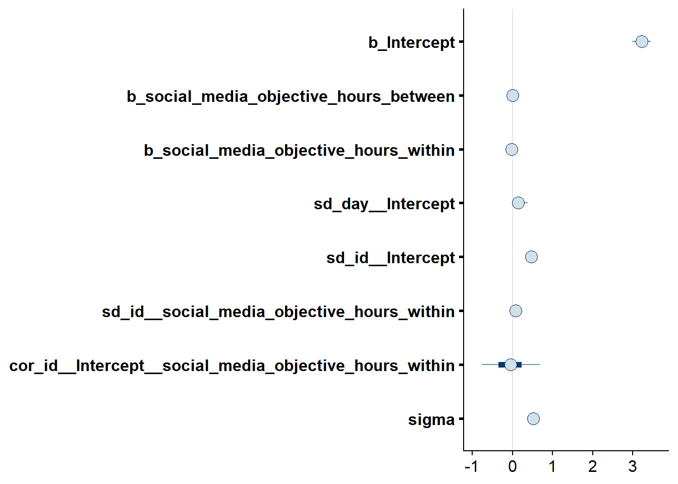

The effects plot (Figure 4.62) visually confirms what I wrote above.

Figure 4.62: Effects plot for Model 7

4.5.2 Model 8: Subjective use predicting well-being

Next, we’ll predict well-being on that day with subjective social media use on that day. There’s conflicting information in the literature: I’m aware of a paper that says subjective estimates overstate the relation, but of another that says the opposite. Therefore,

The specific priors:

For the intercept, I’ll use the same prior as with Model 7.
As for the slopes: This paper reports median effect sizes across all specifications of \(\beta\) = -.08, with effect sizes larger on the between-level, but small to negligible on the within-level. That’s among adolescents and for a longer time frame. This explicitly compared subjective to objective and found that subjective is a much stronger predictor (up to four times the effect size). This says subjective estimates ever so slightly understimate relations between use and well-being, though. Overall, I’d say we can expect a somewhat more negative between-person relation, which would lead us to believe a mean negative effect of -.20 Likert-points on well-being and 0.4 standard deviation to allow for more extreme slopes. That would bring 95% of effects within -1 and 0.6 Likert-points, which is rather generous for media effects.
For the within-effect, I’ll stick to the same prior as for the previous model.
For everything else, I’ll once more go with the default brms priors.

Let’s set those priors.

# set priors
priors_model8 <- 
  c(
    # intercept
    prior(normal(3, 1), class = Intercept),
    
    # slopes for between
    prior(normal(-0.2, 0.4), class = b, coef = "social_media_subjective_hours_between"),
    
    # slopes for between
    prior(normal(0, 0.40), class = b, coef = "social_media_subjective_hours_within")
  )

Okay, let’s run the model.

model8 <- 
  brm(
    data = dat,
    family = gaussian,
    prior = priors_model8,
    well_being_state ~
      1 +
      social_media_subjective_hours_between +
      social_media_subjective_hours_within +
      (
        1 +
        social_media_subjective_hours_within |
        id
      ) +
      (1 |day),
    iter = 5000,
    warmup = 2000,
    chains = 4,
    cores = 4,
    seed = 42,
    control = list(
      adapt_delta = 0.99
    ),
    file = here("models", "model8")
  )

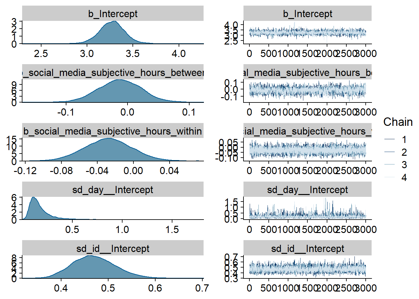
Overall, the traceplots look fine and the chains seem to have mixed well, see (Figure ??).

Figure 4.63: Traceplots and posterior distributions for Model 8

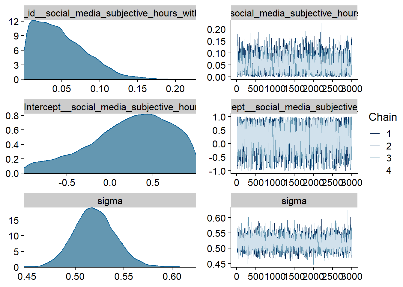
Figure 4.64: Traceplots and posterior distributions for Model 8

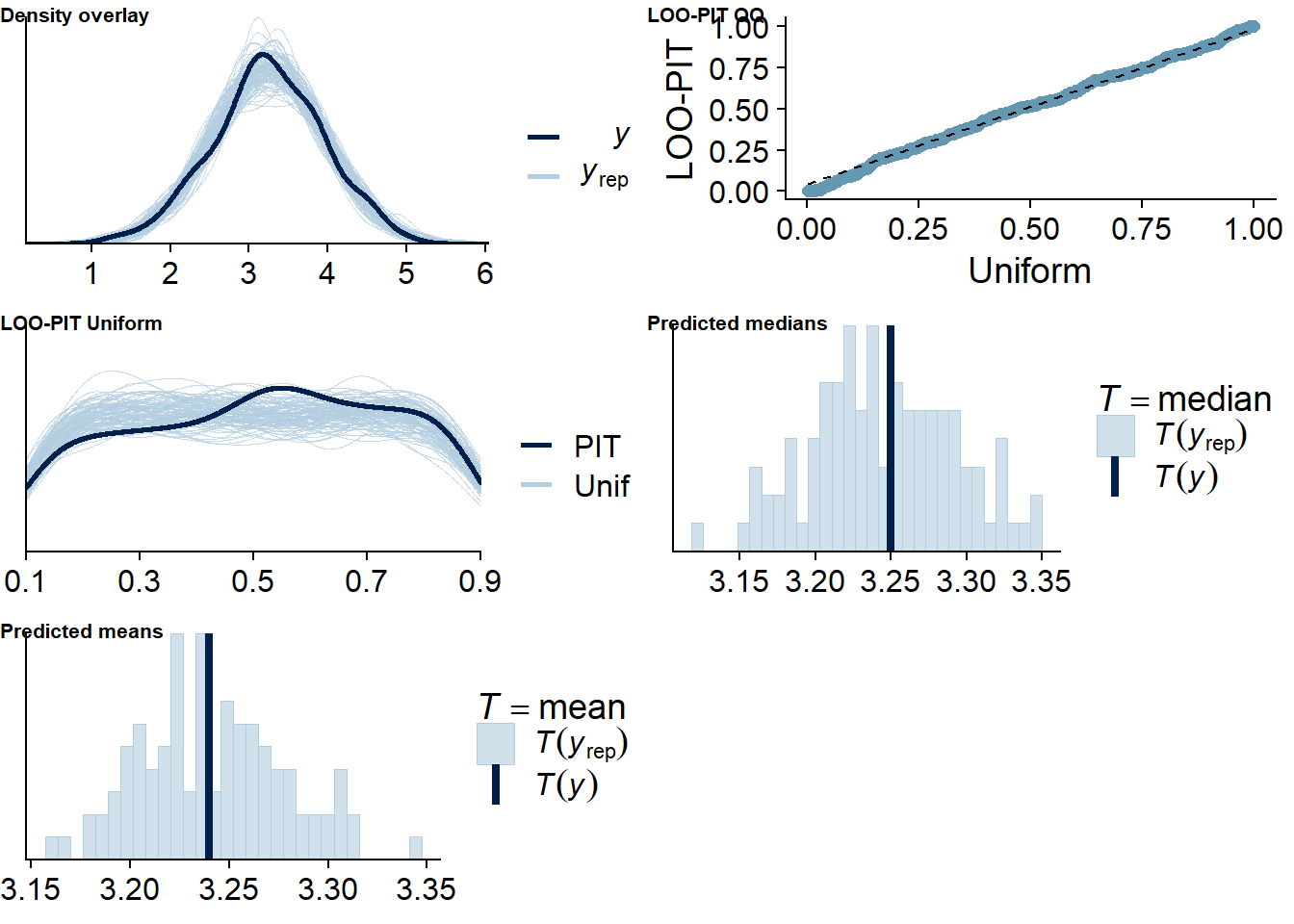
The posterior predictive checks (Figure 4.65) look excellent, just like with Model 7 (no surprise with only one predictor).

Figure 4.65: Posterior predictive checks for Model 8

One case is flagged as potentially influential, but unproblematic after being calculated directly..

loo(model8, reloo = TRUE)

## 1 problematic observation(s) found.
## The model will be refit 1 times.

## 
## Fitting model 1 out of 1 (leaving out observation 413)

## Start sampling

## 
## Computed from 12000 by 425 log-likelihood matrix
## 
##          Estimate   SE
## elpd_loo   -371.1 16.2
## p_loo        78.7  5.4
## looic       742.2 32.4
## ------
## Monte Carlo SE of elpd_loo is 0.2.
## 
## Pareto k diagnostic values:
##                          Count Pct.    Min. n_eff
## (-Inf, 0.5]   (good)     405   95.3%   389       
##  (0.5, 0.7]   (ok)        20    4.7%   554       
##    (0.7, 1]   (bad)        0    0.0%   <NA>      
##    (1, Inf)   (very bad)   0    0.0%   <NA>      
## 
## All Pareto k estimates are ok (k < 0.7).
## See help('pareto-k-diagnostic') for details.

Let’s inspect the summary. The within effect is estimated to be negative, but extremely small. Also, the 95% CI includes zero, so we can’t be sure the effect is meaningful.

summary(model8, priors = TRUE)

##  Family: gaussian 
##   Links: mu = identity; sigma = identity 
## Formula: well_being_state ~ 1 + social_media_subjective_hours_between + social_media_subjective_hours_within + (1 + social_media_subjective_hours_within | id) + (1 | day) 
##    Data: study1 (Number of observations: 425) 
## Samples: 4 chains, each with iter = 5000; warmup = 2000; thin = 1;
##          total post-warmup samples = 12000
## 
## Priors: 
## b_social_media_subjective_hours_between ~ normal(-0.2, 0.4)
## b_social_media_subjective_hours_within ~ normal(0, 0.4)
## Intercept ~ normal(3, 1)
## L ~ lkj_corr_cholesky(1)
## sd ~ student_t(3, 0, 2.5)
## sigma ~ student_t(3, 0, 2.5)
## 
## Group-Level Effects: 
## ~day (Number of levels: 5) 
##               Estimate Est.Error l-95% CI u-95% CI Rhat Bulk_ESS Tail_ESS
## sd(Intercept)     0.18      0.13     0.05     0.51 1.00     2790     3833
## 
## ~id (Number of levels: 94) 
##                                                     Estimate Est.Error l-95% CI u-95% CI Rhat Bulk_ESS Tail_ESS
## sd(Intercept)                                           0.47      0.05     0.39     0.57 1.00     3971     6987
## sd(social_media_subjective_hours_within)                0.05      0.03     0.00     0.13 1.00     3070     4785
## cor(Intercept,social_media_subjective_hours_within)     0.23      0.47    -0.83     0.95 1.00     8042     5984
## 
## Population-Level Effects: 
##                                       Estimate Est.Error l-95% CI u-95% CI Rhat Bulk_ESS Tail_ESS
## Intercept                                 3.27      0.14     2.99     3.55 1.00     3189     4864
## social_media_subjective_hours_between    -0.01      0.04    -0.08     0.06 1.00     3174     5245
## social_media_subjective_hours_within     -0.03      0.03    -0.08     0.02 1.00    12266     8541
## 
## Family Specific Parameters: 
##       Estimate Est.Error l-95% CI u-95% CI Rhat Bulk_ESS Tail_ESS
## sigma     0.52      0.02     0.48     0.56 1.00     9007     8503
## 
## Samples were drawn using sampling(NUTS). For each parameter, Bulk_ESS
## and Tail_ESS are effective sample size measures, and Rhat is the potential
## scale reduction factor on split chains (at convergence, Rhat = 1).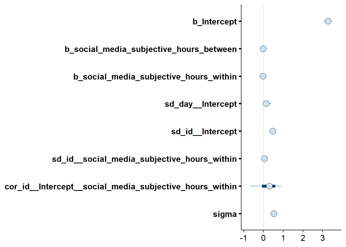

The effects plot (Figure 4.66) shows that the effect, if even there, is small at best.

Figure 4.66: Effects plot for Model 8

4.5.3 Model 9: Accuracy predicting well-being

For this model, we ask whether the error people make in their estimation is related to their well-being on the state level. As for as I know, there’s little prior knowledge we could build on for the relation between accuracy and well-being.

As for the specific priors:

Like before, at perfect accuracy (0% error) and zero deviation I’ll assume a normal distribution centered on the midpoint of the scale (i.e., 3) with the intercept. I’ll set the SD of that prior distribution to 1 once more.
As for the slopes: There’s one paper that correlated the absolute discrepancy between subjective and objective social media use and well-being indicators aggregated over a week. They found a \(\beta\) = .16 between log-transformed discrepancies and depression scores. Discrepancy is a different measurement than the error that we calculated for accuracy. Therefore, I’ll use a prior that’s centered on a negative relationship with a small SD. Like above, I don’t expect that there will be large effects just based on the literature. So I’ll assume a small effect (say -0.20 Likert-scales) with a somewhat wider standard deviation than in previous models (say 0.4). This way, 95% of effects will be within -1 (-.20 + (2 times 0.3)) and 0.60 Likert-points on the outcome scale. However, error is in percent, so we wouldn’t expect -.20 Likert-points with every one-percent increase. Rather, I’d say the above effect is easier to specify for a standard deviation change in error, which is why I standardize error: one standard deviation increase in accuracy will be associated with, on average, a .20 lower score on well-being on the between level.
I have no information for the within-level, which is why I use a prior centered on zero with the same wide standard deviation.
For everything else, I’ll once more go with the default brms priors.

Let’s set those priors and center at the same time.

# standardize error
dat <- 
  dat %>% 
  mutate(
    error_s = scale(error, center = FALSE, scale = TRUE)
  )

# center to get between and within
dat <- 
  dat %>% 
  group_by(id) %>% 
  mutate(
    across(
      error_s,
      list(
        between = ~ mean(.x, na.rm = TRUE),
        within = ~.x - mean(.x, na.rm = TRUE)
      )
    )
  ) %>% 
  ungroup()

# set priors
priors_model9 <- 
  c(
    # intercept
    prior(normal(3, 1), class = Intercept),
    
    # slopes for between
    prior(normal(-0.2, 0.4), class = b, coef = "error_s_between"),
    
    # slopes for between
    prior(normal(0, 0.40), class = b, coef = "error_s_within")
  )

And run the model.

model9 <- 
  brm(
    data = dat,
    family = gaussian,
    prior = priors_model9,
    well_being_state ~
      1 +
      error_s_between +
      error_s_within +
      (
        1 +
        error_s_within |
        id
      ) +
      (1 |day),
    iter = 5000,
    warmup = 2000,
    chains = 4,
    cores = 4,
    seed = 42,
    control = list(
      adapt_delta = 0.999
    ),
    file = here("models", "model9")
  )

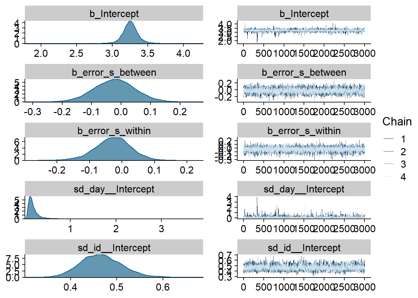
Overall, the traceplots look fine and the chains seem to have mixed well, see (Figure ??).

Figure 4.67: Traceplots and posterior distributions for Model 9

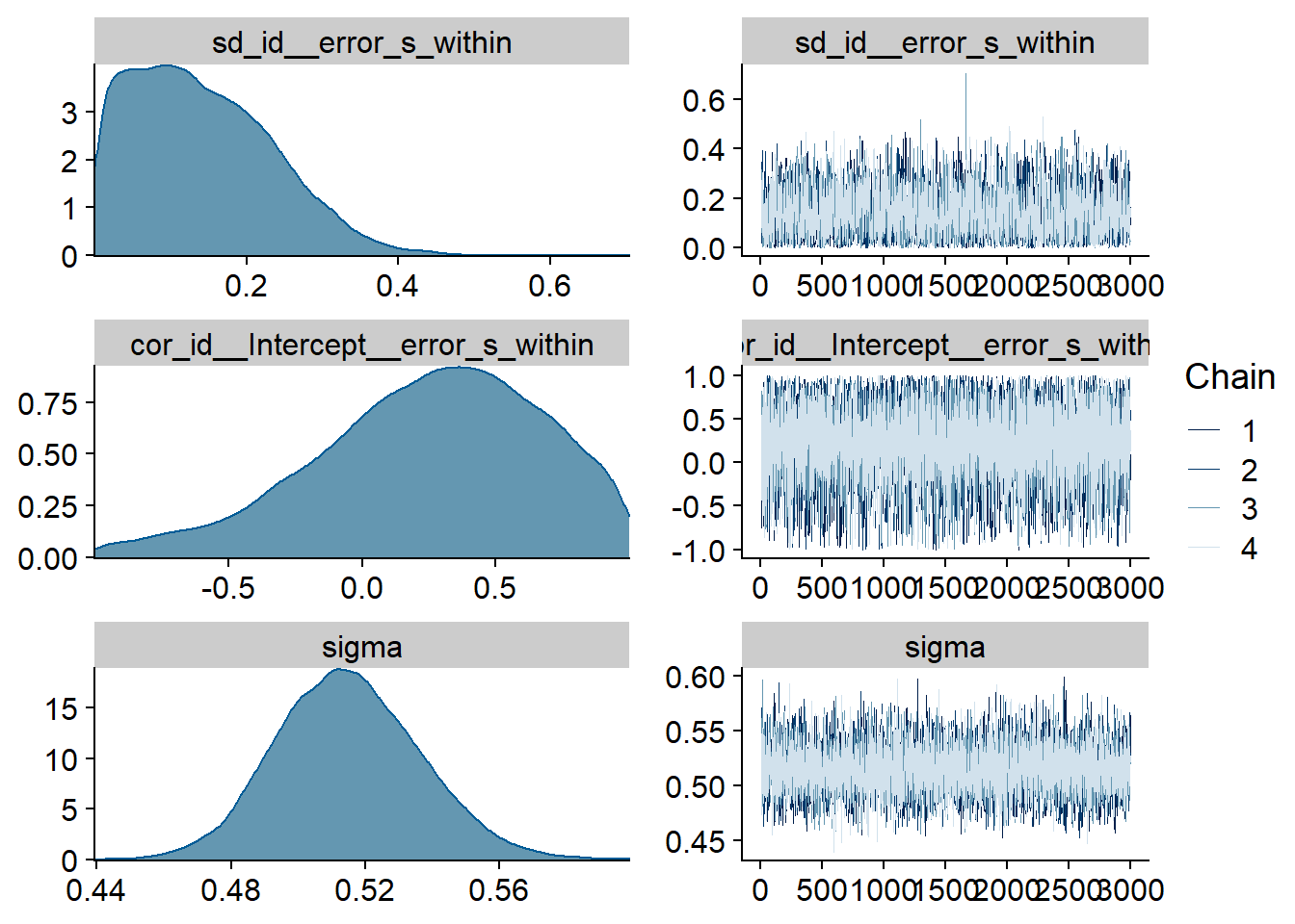
Figure 4.68: Traceplots and posterior distributions for Model 9

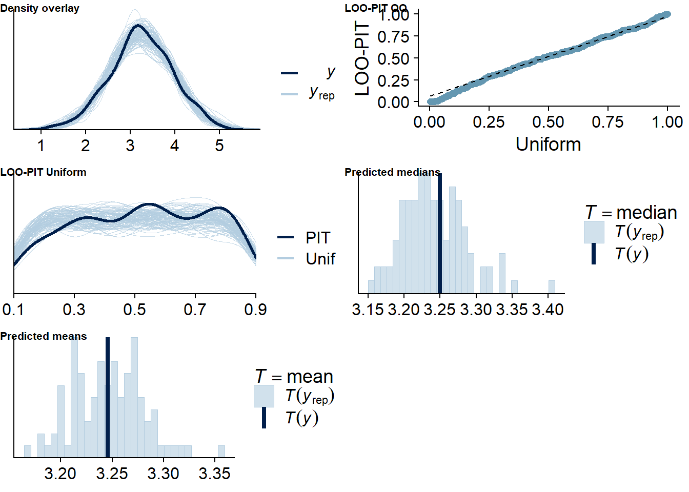
The posterior predictive checks (Figure 4.69) look excellent (no surprise with only one predictor).

Figure 4.69: Posterior predictive checks for Model 9

Six cases are flagged as potentially influential, which is why we calculate ELPD directly.

loo(model9, reloo = TRUE)

## 6 problematic observation(s) found.
## The model will be refit 6 times.

## 
## Fitting model 1 out of 6 (leaving out observation 23)

## 
## Fitting model 2 out of 6 (leaving out observation 24)

## 
## Fitting model 3 out of 6 (leaving out observation 255)

## 
## Fitting model 4 out of 6 (leaving out observation 289)

## 
## Fitting model 5 out of 6 (leaving out observation 397)

## 
## Fitting model 6 out of 6 (leaving out observation 417)

## Start sampling
## Start sampling
## Start sampling
## Start sampling
## Start sampling
## Start sampling

## 
## Computed from 12000 by 423 log-likelihood matrix
## 
##          Estimate   SE
## elpd_loo   -367.8 16.4
## p_loo        81.4  6.0
## looic       735.6 32.8
## ------
## Monte Carlo SE of elpd_loo is 0.2.
## 
## Pareto k diagnostic values:
##                          Count Pct.    Min. n_eff
## (-Inf, 0.5]   (good)     407   96.2%   47        
##  (0.5, 0.7]   (ok)        16    3.8%   492       
##    (0.7, 1]   (bad)        0    0.0%   <NA>      
##    (1, Inf)   (very bad)   0    0.0%   <NA>      
## 
## All Pareto k estimates are ok (k < 0.7).
## See help('pareto-k-diagnostic') for details.

Let’s inspect the summary. The within effect is estimated to be negative, but really small. Also, the 95% CI includes zero and quite wide, so we can’t be sure the effect is meaningful.

summary(model9, priors = TRUE)

##  Family: gaussian 
##   Links: mu = identity; sigma = identity 
## Formula: well_being_state ~ 1 + error_s_between + error_s_within + (1 + error_s_within | id) + (1 | day) 
##    Data: study1 (Number of observations: 423) 
## Samples: 4 chains, each with iter = 5000; warmup = 2000; thin = 1;
##          total post-warmup samples = 12000
## 
## Priors: 
## b_error_s_between ~ normal(-0.2, 0.4)
## b_error_s_within ~ normal(0, 0.4)
## Intercept ~ normal(3, 1)
## L ~ lkj_corr_cholesky(1)
## sd ~ student_t(3, 0, 2.5)
## sigma ~ student_t(3, 0, 2.5)
## 
## Group-Level Effects: 
## ~day (Number of levels: 5) 
##               Estimate Est.Error l-95% CI u-95% CI Rhat Bulk_ESS Tail_ESS
## sd(Intercept)     0.19      0.15     0.06     0.53 1.00     3196     3812
## 
## ~id (Number of levels: 94) 
##                               Estimate Est.Error l-95% CI u-95% CI Rhat Bulk_ESS Tail_ESS
## sd(Intercept)                     0.47      0.04     0.39     0.56 1.00     4652     8200
## sd(error_s_within)                0.14      0.09     0.01     0.34 1.00     2730     5295
## cor(Intercept,error_s_within)     0.25      0.42    -0.72     0.93 1.00     9691     7015
## 
## Population-Level Effects: 
##                 Estimate Est.Error l-95% CI u-95% CI Rhat Bulk_ESS Tail_ESS
## Intercept           3.25      0.13     3.01     3.48 1.00     4066     3419
## error_s_between    -0.02      0.07    -0.16     0.12 1.00     6313     7487
## error_s_within     -0.03      0.06    -0.15     0.08 1.00    13197     8720
## 
## Family Specific Parameters: 
##       Estimate Est.Error l-95% CI u-95% CI Rhat Bulk_ESS Tail_ESS
## sigma     0.51      0.02     0.48     0.56 1.00     9411     9387
## 
## Samples were drawn using sampling(NUTS). For each parameter, Bulk_ESS
## and Tail_ESS are effective sample size measures, and Rhat is the potential
## scale reduction factor on split chains (at convergence, Rhat = 1).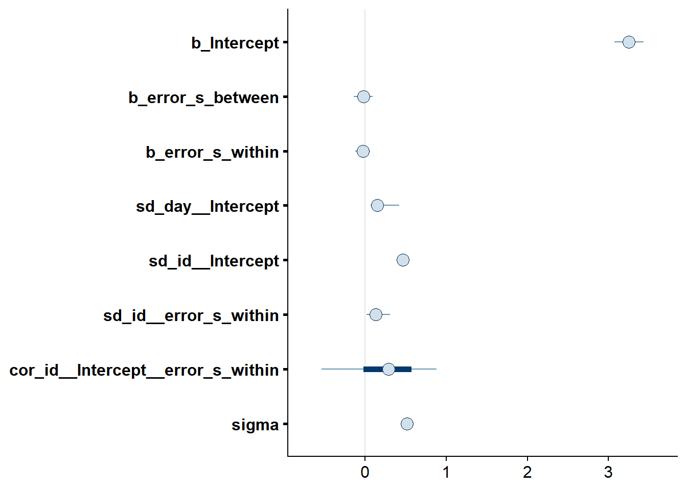

The effects plot (Figure 4.70) shows that the effect, if even there, is small at best.

Figure 4.70: Effects plot for Model 9

4.6 Relation between subjective and objective use

Something that wasn’t part of the original plan: inspecting the relation between subjective and objective use a bit closer. The absolute difference between the two wasn’t that large, so it’s possible that the difference isn’t meaningfully different from zero. For that reason, I predict subjective use with objective use and then inspect the parameter. The intercept will tell us whether the subjective overestimate is different from zero (so an indicator of bias). The slope will tell us how sensitive subjective is to the true value. And the sigma will tell us how much error there is.

Unfortunately, the model has huge problems with a Gamma distribution as outcome, so I went for a normal distribution with the predictor grand-mean centered instead. Also, I’m not using informed priors here and rely on the default brms priors. For this question, I’m not interested in distinguishing between- and within-person effects.

model10 <- 
  brm(
    data = dat,
    family = gaussian,
    social_media_subjective ~
      1 +
      social_media_objective +
      (1 + social_media_objective | id) +
      (1 | day),
    iter = 5000,
    warmup = 2000,
    chains = 4,
    cores = 4,
    seed = 42,
    control = list(adapt_delta = 0.99),
    file = here("models", "model10.rds")
  )

Overall, the traceplots look fine and the chains seem to have mixed well, see (Figure ??).

Figure 4.71: Traceplots and posterior distributions for Model 10

Figure 4.72: Traceplots and posterior distributions for Model 10

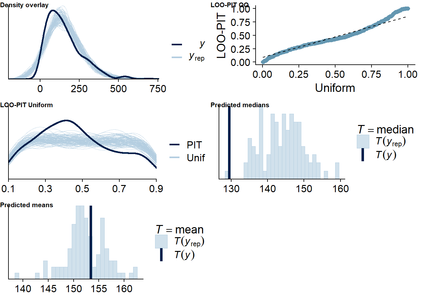
The posterior predictive checks (Figure 4.73) look good, but overestimating how many negative values there are because it relies on a normal distribution.

Figure 4.73: Posterior predictive checks for Model 10

Five cases are flagged as potentially influential, which is why we calculate ELPD directly.

loo(model10, reloo = TRUE)

## 5 problematic observation(s) found.
## The model will be refit 5 times.

## 
## Fitting model 1 out of 5 (leaving out observation 23)

## 
## Fitting model 2 out of 5 (leaving out observation 63)

## 
## Fitting model 3 out of 5 (leaving out observation 134)

## 
## Fitting model 4 out of 5 (leaving out observation 350)

## 
## Fitting model 5 out of 5 (leaving out observation 392)

## Start sampling
## Start sampling
## Start sampling
## Start sampling
## Start sampling

## 
## Computed from 12000 by 428 log-likelihood matrix
## 
##          Estimate   SE
## elpd_loo  -2439.9 23.7
## p_loo        85.1  8.2
## looic      4879.8 47.4
## ------
## Monte Carlo SE of elpd_loo is 0.3.
## 
## Pareto k diagnostic values:
##                          Count Pct.    Min. n_eff
## (-Inf, 0.5]   (good)     401   93.7%   39        
##  (0.5, 0.7]   (ok)        27    6.3%   134       
##    (0.7, 1]   (bad)        0    0.0%   <NA>      
##    (1, Inf)   (very bad)   0    0.0%   <NA>      
## 
## All Pareto k estimates are ok (k < 0.7).
## See help('pareto-k-diagnostic') for details.

Let’s inspect the summary: indeed the intercept is different from zero, which speaks for a bias/systematic error in overestimates of social media time.

summary(model10, priors = TRUE)

##  Family: gaussian 
##   Links: mu = identity; sigma = identity 
## Formula: social_media_subjective ~ 1 + social_media_objective + (1 + social_media_objective | id) + (1 | day) 
##    Data: study1 (Number of observations: 428) 
## Samples: 4 chains, each with iter = 5000; warmup = 2000; thin = 1;
##          total post-warmup samples = 12000
## 
## Priors: 
## Intercept ~ student_t(3, 129.5, 103)
## L ~ lkj_corr_cholesky(1)
## sd ~ student_t(3, 0, 103)
## sigma ~ student_t(3, 0, 103)
## 
## Group-Level Effects: 
## ~day (Number of levels: 5) 
##               Estimate Est.Error l-95% CI u-95% CI Rhat Bulk_ESS Tail_ESS
## sd(Intercept)     4.99      5.52     0.15    18.65 1.00     6023     6603
## 
## ~id (Number of levels: 94) 
##                                       Estimate Est.Error l-95% CI u-95% CI Rhat Bulk_ESS Tail_ESS
## sd(Intercept)                            57.35     10.50    37.79    79.11 1.00     4648     7538
## sd(social_media_objective)                0.22      0.09     0.06     0.40 1.00      960     2260
## cor(Intercept,social_media_objective)     0.10      0.42    -0.57     0.93 1.00     1411     2450
## 
## Population-Level Effects: 
##                        Estimate Est.Error l-95% CI u-95% CI Rhat Bulk_ESS Tail_ESS
## Intercept                 71.21     11.16    49.54    92.95 1.00     8331     9048
## social_media_objective     0.59      0.07     0.45     0.72 1.00    10561     8913
## 
## Family Specific Parameters: 
##       Estimate Est.Error l-95% CI u-95% CI Rhat Bulk_ESS Tail_ESS
## sigma    64.24      2.57    59.45    69.44 1.00     7416     8846
## 
## Samples were drawn using sampling(NUTS). For each parameter, Bulk_ESS
## and Tail_ESS are effective sample size measures, and Rhat is the potential
## scale reduction factor on split chains (at convergence, Rhat = 1).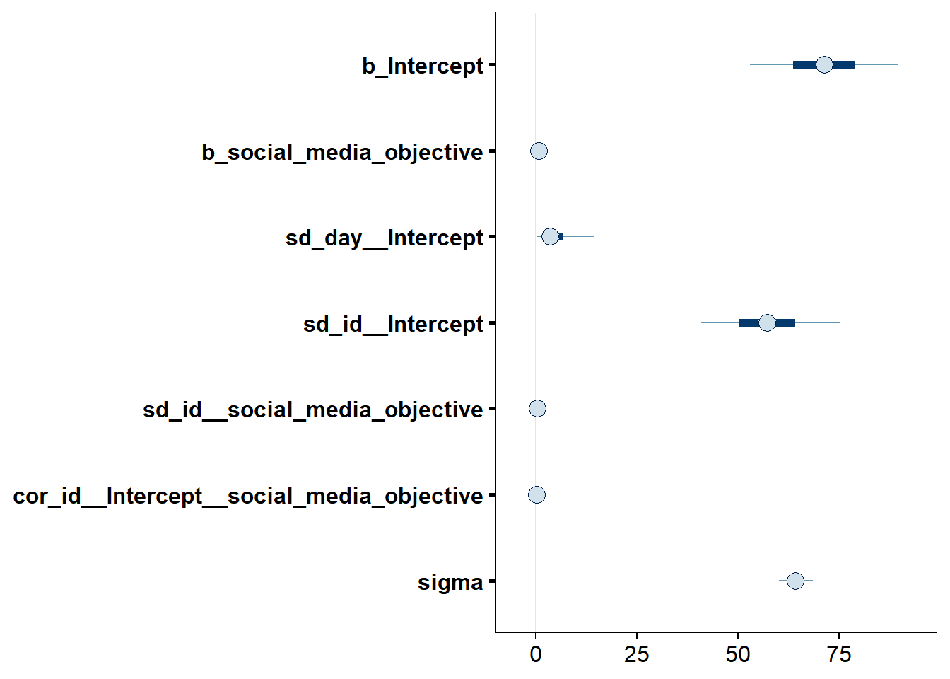

The effects plot (Figure 4.74) shows that visually.

Figure 4.74: Effects plot for Model 10