4  Study 2: Gaming and Sleep

if (!require("pacman")) install.packages("pacman")
library(pacman)

p_load(tidyverse, lme4, marginaleffects, glmmTMB, mice, ordinal, modelsummary, lubridate, data.table)

studyStartDate <- as_datetime("2024-05-01 00:00:00")

# don't use read_csv for the synPanelClean! no idea why but it guesses column
# type wrong, leading to a lot of NA imports

data.panel <- fread("data/data-synthetic-clean/synPanelClean.csv.gz") |> # requires that the preprocessing script has been run
  left_join(read_csv("data/data-synthetic-clean/synIntakeClean.csv.gz"), by = "pid") |> 
  dplyr::select(pid, wave, region, psqi_6, starts_with(c("mctq", "eps", "psqi")), total_hours_sleep, wemwbs, 
         age_scaled, bmi_scaled, SES_index_scaled, msf_sc_numeric, gender) |> 
  mutate(
    psqi_6_ord = factor(psqi_6, ordered = TRUE),
    pid = as.character(pid)
  )

data.nin <- read_csv("data/data-synthetic-clean/synNintendoClean.csv.gz")
data.xbox <- read_csv("data/data-synthetic-clean/synXboxClean.csv.gz")
data.steam <- read_csv("data/data-synthetic-clean/synSteamClean.csv.gz")
data.android <- read_csv("data/data-synthetic-raw/synAndroid.csv.gz")
data.ios <- read_csv("data/data-synthetic-raw/syniOS.csv.gz")

# merge xbox_balanced and steam_balanced and nin_balanced 
data.gaming <- bind_rows(data.xbox, data.steam, data.nin) |> 
  
  mutate(
    
    # redefine day to begin and end at 4am, rather than midnight, so we can properly
    # assign late-night sessions to the previous calendar day
    dateRecoded = if_else(hour(sessionStart) < 6, date - 1, date),
    
    # calculate minutes_played for data.gaming using sessionEnd and sessionStart
    # create a binary variable for data.gaming called latenight if the sessionStart is between 23:00 and 06:00
    # create an isWeekend variable for data.gaming if the sessionStart is on a Saturday, Sunday or Friday
    minutes_played = as.numeric(difftime(sessionEnd, sessionStart, units = "mins")),
    latenight = ifelse(hour(sessionStart) >= 23 | hour(sessionStart) < 6, 1, 0),
    isWeekend = ifelse(weekdays(sessionStart) %in% c("Friday", "Saturday"), 1, 0),
    
    # calculate late night using lubridate::interval objects
    interval_gaming = interval(sessionStart, sessionEnd),
    interval_latenight = interval(dateRecoded + hours(23), dateRecoded + hours(30)), # gets the 11pm to 6am following day interval from date
    latenightMinutes = as.numeric(intersect(interval_gaming, interval_latenight))/60 # calculate overlap in minutes
  ) |> 

  # assign each session to a wave based on the date, if the date is within 4
  # weeks of the start of the study, it is wave 2, if it is between 4 weeks and
  # 8 weeks it is wave 4, if it is between 8 weeks and 12 weeks it is wave 6
  mutate(
    days_since_start = as.numeric(difftime(sessionStart, studyStartDate, units = "days")),
    month = case_when(
      day >= 0 & day <= 28 ~ 2,
      day >= 29 & day <= 56 ~ 4,
      day >= 57 & day <= 84 ~ 6,
      TRUE ~ NA_real_
    ),
    # Define biweekly waves (14-day intervals) that end at day 84
    wave = case_when(
      day >= 0 & day <= 14 ~ 1,
      day >= 15 & day <= 28 ~ 2,
      day >= 29 & day <= 42 ~ 3,
      day >= 43 & day <= 56 ~ 4,
      day >= 57 & day <= 70 ~ 5,
      day >= 71 & day <= 84 ~ 6,
      TRUE ~ NA_real_  # Assign NA for days beyond 84
    ),
    pid = as.character(pid)
  ) 

# group gaming by PID, wave and latenight and calculate daily average minutes_played
gamingMonthly <- data.gaming |> 
  group_by(pid, month, isWeekend) %>%
  summarise(
    monthly_avg_minutes_played = sum(latenightMinutes)/28,
  ) |> 
  left_join(data.panel |> dplyr::select(-msf_sc_numeric) |> filter(wave %in% c(2, 4, 6)), 
            by = c("pid","month" = "wave")) |> 
  left_join(data.panel |> dplyr::select(pid, msf_sc_numeric) |> filter(!is.na(msf_sc_numeric)), 
            by = c("pid")) |> # hacky way to make sure chronotype (measured in wave 1 only) doesn't get lost 
  mutate(monthly_avg_minutes_played = replace_na(monthly_avg_minutes_played, 0)) |> 
  ungroup() |>
  arrange(as.integer(pid), month)

# group gaming by PID, wave and latenight and calculate daily average minutes_played
gamingBiweekly <- data.gaming |> 
  group_by(pid, wave, isWeekend) |> 
  summarise(
    biweekly_avg_minutes_played = sum(latenightMinutes)/14,
  ) |> 
  left_join(data.panel |> dplyr::select(-msf_sc_numeric), by = c("pid", "wave")) |> 
  left_join(data.panel |> dplyr::select(pid, msf_sc_numeric) |> filter(!is.na(msf_sc_numeric)), 
            by = c("pid")) |> # hacky way to make sure chronotype (measured in wave 1 only) doesn't get lost 
  mutate(biweekly_avg_minutes_played = replace_na(biweekly_avg_minutes_played, 0)) |> 
  ungroup() |> 
  arrange(as.integer(pid), wave) |> 
  dplyr::select(pid, wave, msf_sc_numeric, everything())

4.1 H1a: Late-night gaming is associated with poorer sleep quality.

Multilevel ordinal regression whereby monthly average minutes played predicts sleep quality (PSQI), controlling for age, BMI, SES index, region, and whether playtime falls on a weekend, with a random intercept and slope for participants.

# For psqi_6 1 means Very good, 2 means Fairly good, 3 means Fairly bad, 4 means Very bad

# Fit the model with rescaled covariates
model.h1a <- clmm(psqi_6_ord ~ monthly_avg_minutes_played + (1 + monthly_avg_minutes_played | pid) +
                    age_scaled + bmi_scaled + SES_index_scaled + region + isWeekend,
                  data = gamingMonthly)

modelsummary(
  list(`Model H1a` = model.h1a),
  fmt = 2,
  estimate  = "{estimate} [{conf.low}, {conf.high}]{stars}", 
  statistic = NULL
)

	Model H1a
1|2	-1.45 [-1.61, -1.29]***
2|3	0.00 [-0.16, 0.16]
3|4	1.49 [1.33, 1.65]***
monthly_avg_minutes_played	0.06 [-0.01, 0.13]+
age_scaled	-0.12 [-0.24, 0.00]*
bmi_scaled	0.04 [-0.04, 0.13]
SES_index_scaled	0.07 [-0.02, 0.16]
regionUS	-0.11 [-0.35, 0.12]
isWeekend	-0.01 [-0.11, 0.08]
SD (Intercept pid)	1.40
SD (monthly_avg_minutes_played pid)	0.00
Cor (Intercept~monthly_avg_minutes_played pid)	-1.00
Num.Obs.	6329
R2 Marg.	0.005
AIC	16748.6
BIC	16829.7
RMSE	2.39

4.2 H1b: Late-night gaming is associated with shorter sleep duration.

Multilevel linear regression whereby monthly average minutes played predicts total hours of sleep (PSQI), controlling for age, BMI, SES index, region, gender, and whether playtime falls on a weekend, with a random intercept and slope for participants and a random intercept for gender.

# Fit the model
model.h1b <- lmer(total_hours_sleep ~ monthly_avg_minutes_played + (1 + monthly_avg_minutes_played | pid) +
                    age_scaled + bmi_scaled + SES_index_scaled + (1 | gender) + region + isWeekend, 
                  data = gamingMonthly
                  )

# Summarize the model using modelsummary
modelsummary(
  list(`Model H1b` = model.h1b),
  fmt = 2,
  estimate  = "{estimate} [{conf.low}, {conf.high}]{stars}", 
  statistic = NULL
)

	Model H1b
(Intercept)	6.63 [6.41, 6.85]***
monthly_avg_minutes_played	-0.07 [-0.18, 0.04]
age_scaled	-0.08 [-0.25, 0.09]
bmi_scaled	-0.02 [-0.15, 0.10]
SES_index_scaled	-0.03 [-0.15, 0.10]
regionUS	-0.05 [-0.39, 0.29]
isWeekend	0.04 [-0.10, 0.19]
SD (Intercept pid)	1.96
SD (monthly_avg_minutes_played pid)	0.09
Cor (Intercept~monthly_avg_minutes_played pid)	1.00
SD (Intercept gender)	0.00
SD (Observations)	2.92
Num.Obs.	6329
R2 Marg.	0.001
R2 Cond.	0.313
AIC	33147.6
BIC	33228.7
ICC	0.3
RMSE	2.69

4.3 H1c: Late-night gaming is associated with lower well-being.

Multilevel linear regression whereby monthly average minutes played predicts daytime sleepiness (Epworth Sleepiness Scale), controlling for age, BMI, SES index, region, gender, and whether playtime falls on a weekend, with a random intercept and slope for participants and a random intercept for gender.

model.h1c <- lmer(wemwbs ~ biweekly_avg_minutes_played + (1 + biweekly_avg_minutes_played | pid) +
                    age_scaled + bmi_scaled + SES_index_scaled + (1 | gender) + region + isWeekend, 
                  data = gamingBiweekly)

modelsummary(
  list(`Model H1c` = model.h1c),
  fmt = 2,
  estimate  = "{estimate} [{conf.low}, {conf.high}]{stars}", 
  statistic = NULL
)

	Model H1c
(Intercept)	2.98 [2.96, 3.00]***
biweekly_avg_minutes_played	0.00 [0.00, 0.00]
age_scaled	0.02 [0.00, 0.04]+
bmi_scaled	0.01 [0.00, 0.02]+
SES_index_scaled	0.00 [-0.01, 0.02]
regionUS	0.03 [0.00, 0.07]+
isWeekend	0.00 [-0.02, 0.02]
SD (Intercept pid)	0.19
SD (biweekly_avg_minutes_played pid)	0.00
Cor (Intercept~biweekly_avg_minutes_played pid)	1.00
SD (Intercept gender)	0.00
SD (Observations)	0.50
Num.Obs.	12598
R2 Marg.	0.001
AIC	19675.6
BIC	19764.9
RMSE	0.48

4.4 H1d: Late-night gaming is associated with higher daytime sleepiness.

Multilevel linear regression whereby biweekly average minutes played predicts well-being (WEMWBS), controlling for age, BMI, SES index, region, gender, and whether playtime falls on a weekend, with a random intercept and slope for participants and a random intercept for gender.

# Fit the model
model.h1d <- lmer(epsTotal ~ monthly_avg_minutes_played + (1 + monthly_avg_minutes_played | pid) +
                    age_scaled + bmi_scaled + SES_index_scaled + (1 | gender) + region + isWeekend, 
                  data = gamingMonthly)

# Summarize the model using modelsummary
modelsummary(
  list(`Model H1d` = model.h1d),
  fmt = 2,
  estimate  = "{estimate} [{conf.low}, {conf.high}]{stars}", 
  statistic = NULL
)

	Model H1d
(Intercept)	7.06 [6.69, 7.43]***
monthly_avg_minutes_played	-0.07 [-0.18, 0.05]
age_scaled	0.06 [-0.24, 0.35]
bmi_scaled	0.09 [-0.12, 0.30]
SES_index_scaled	-0.09 [-0.30, 0.12]
regionUS	0.24 [-0.34, 0.82]
isWeekend	0.00 [-0.18, 0.19]
SD (Intercept pid)	4.19
SD (monthly_avg_minutes_played pid)	0.05
Cor (Intercept~monthly_avg_minutes_played pid)	1.00
SD (Intercept gender)	0.00
SD (Observations)	4.86
Num.Obs.	10650
R2 Marg.	0.001
AIC	67015.7
BIC	67102.9
RMSE	4.50

4.5 H2

4.5.1 H2a: The negative association between late-night gaming and sleep quality is more pronounced among evening chronotypes.

Multilevel ordinal regression whereby the interaction between monthly average minutes played and chronotype (MSFsc: mid-sleep on free days corrected for sleep debt on weekdays; MCTQ) predicts sleep quality (PSQI), controlling for age, BMI, SES index, region, and whether playtime falls on a weekend, with a random intercept and slope for participants.

On the simulation data, there are convergence problems, so here we center late night minutes and chronotype. This will either be uncentered for interpretation or not necessary on the true data.)

# Fit the model with rescaled covariates
model.h2a <- clmm(psqi_6_ord ~ scale(monthly_avg_minutes_played) * scale(msf_sc_numeric) + (1 + monthly_avg_minutes_played | pid) +
                    age_scaled + bmi_scaled + SES_index_scaled + region + isWeekend,
                  data = gamingMonthly)

modelsummary(
  list(`Model H2a` = model.h2a),
  fmt = 2,
  estimate  = "{estimate} [{conf.low}, {conf.high}]{stars}", 
  statistic = NULL
)

	Model H2a
1|2	-1.28 [-1.53, -1.04]***
2|3	0.14 [-0.10, 0.38]
3|4	1.63 [1.38, 1.88]***
scale(monthly_avg_minutes_played)	-0.05 [-0.17, 0.07]
scale(msf_sc_numeric)	-0.03 [-0.16, 0.10]
age_scaled	-0.10 [-0.29, 0.09]
bmi_scaled	-0.10 [-0.23, 0.03]
SES_index_scaled	0.02 [-0.11, 0.16]
regionUS	-0.01 [-0.37, 0.36]
isWeekend	-0.01 [-0.15, 0.14]
scale(monthly_avg_minutes_played) × scale(msf_sc_numeric)	-0.04 [-0.14, 0.07]
SD (Intercept pid)	1.38
SD (monthly_avg_minutes_played pid)	0.14
Cor (Intercept~monthly_avg_minutes_played pid)	1.00
Num.Obs.	2661
R2 Marg.	0.005
R2 Cond.	0.369
AIC	7048.3
BIC	7130.7
RMSE	2.36

4.6 H2b: The negative association between late-night gaming and sleep duration is more pronounced among evening chronotypes.

# Fit the model
model.h2b <- lmer(total_hours_sleep ~ monthly_avg_minutes_played * msf_sc_numeric + (1 + monthly_avg_minutes_played | pid) +
                    age_scaled + bmi_scaled + SES_index_scaled + region + isWeekend + (1 | gender), 
                  data = gamingMonthly)

# Summarize the model using modelsummary
modelsummary(
  list(`Model H2b` = model.h2b),
  fmt = 2,
  estimate  = "{estimate} [{conf.low}, {conf.high}]{stars}", 
  statistic = NULL
)

	Model H2b
(Intercept)	6.78 [6.27, 7.28]***
monthly_avg_minutes_played	0.05 [-0.28, 0.38]
msf_sc_numeric	-0.01 [-0.04, 0.02]
age_scaled	-0.21 [-0.48, 0.06]
bmi_scaled	0.02 [-0.18, 0.21]
SES_index_scaled	-0.03 [-0.23, 0.16]
regionUS	-0.07 [-0.60, 0.45]
isWeekend	0.01 [-0.22, 0.24]
monthly_avg_minutes_played × msf_sc_numeric	-0.01 [-0.03, 0.01]
SD (Intercept pid)	1.93
SD (monthly_avg_minutes_played pid)	0.13
Cor (Intercept~monthly_avg_minutes_played pid)	1.00
SD (Intercept gender)	0.21
SD (Observations)	2.95
Num.Obs.	2661
R2 Marg.	0.005
AIC	14000.4
BIC	14082.8
RMSE	2.72

4.6.1 H2c: The negative association between late-night gaming and well-being is more pronounced among evening chronotypes.

Multilevel linear regression whereby the interaction between monthly average minutes played and chronotype (MSFsc; MCTQ) predicts daytime sleepiness (Epworth Sleepiness Scale), controlling for age, BMI, SES index, region, gender, and whether playtime falls on a weekend, with a random intercept and slope for participants and a random intercept for gender.

# Fit the model
model.h2c <- lmer(wemwbs ~ biweekly_avg_minutes_played * msf_sc_numeric + (1 | pid) +
                    age_scaled + bmi_scaled + SES_index_scaled + region + isWeekend + (1 | gender), 
                  data = gamingBiweekly)
modelsummary(
  list(`Model h2c` = model.h2c),
  fmt = 2,
  estimate  = "{estimate} [{conf.low}, {conf.high}]{stars}", 
  statistic = NULL
)

	Model h2c
(Intercept)	3.00 [2.95, 3.06]***
biweekly_avg_minutes_played	0.00 [-0.01, 0.01]
msf_sc_numeric	0.00 [0.00, 0.00]
age_scaled	0.00 [-0.03, 0.03]
bmi_scaled	0.02 [-0.01, 0.04]
SES_index_scaled	0.02 [-0.01, 0.04]
regionUS	0.02 [-0.04, 0.08]
isWeekend	0.00 [-0.03, 0.03]
biweekly_avg_minutes_played × msf_sc_numeric	0.00 [0.00, 0.00]
SD (Intercept pid)	0.21
SD (Intercept gender)	0.00
SD (Observations)	0.50
Num.Obs.	5388
R2 Marg.	0.004
AIC	8543.0
BIC	8622.1
RMSE	0.48

4.6.2 H2d: The negative association between late-night gaming and daytime sleepiness is more pronounced among evening chronotypes.

Multilevel linear regression whereby the interaction between biweekly average minutes played and chronotype (MSFsc; MCTQ) predicts well-being (WEMWBS), controlling for age, BMI, SES index, region, gender, and whether playtime falls on a weekend, with a random intercept for participants and a random intercept for gender.

model.h2d <- lmer(epsTotal ~ monthly_avg_minutes_played * msf_sc_numeric + (1 + monthly_avg_minutes_played | pid) +
                    age_scaled + bmi_scaled + SES_index_scaled + region + isWeekend + (1 | gender), 
                  data = gamingMonthly)
                  
modelsummary(
  list(`Model H2d` = model.h2d),
  fmt = 2,
  estimate  = "{estimate} [{conf.low}, {conf.high}]{stars}", 
  statistic = NULL
)

	Model H2d
(Intercept)	7.42 [6.61, 8.24]***
monthly_avg_minutes_played	-0.19 [-0.50, 0.11]
msf_sc_numeric	-0.02 [-0.06, 0.03]
age_scaled	-0.04 [-0.50, 0.42]
bmi_scaled	0.05 [-0.28, 0.38]
SES_index_scaled	-0.02 [-0.35, 0.31]
regionUS	0.14 [-0.77, 1.04]
isWeekend	0.02 [-0.28, 0.31]
monthly_avg_minutes_played × msf_sc_numeric	0.01 [-0.01, 0.04]
SD (Intercept pid)	4.14
SD (monthly_avg_minutes_played pid)	0.08
Cor (Intercept~monthly_avg_minutes_played pid)	1.00
SD (Intercept gender)	0.00
SD (Observations)	4.89
Num.Obs.	4408
R2 Marg.	0.001
AIC	27796.0
BIC	27885.5
RMSE	4.53

4.7 Precision Analysis

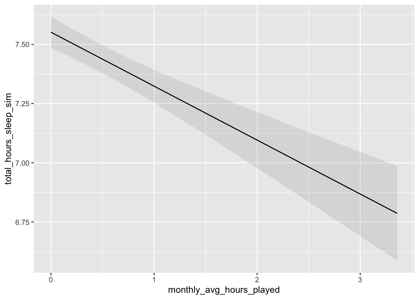
In the above examples, we use the simulated data, which mirrors the structure of the true data, but lacks control over the distribution and relationships between the particular variables used in this study. To provide rough indications of the estimated precision of our tests, here we simulate a dataset with a known relationship between playtime and sleep, and then fit H1b as above (selecting one hypothesis for detailed inspection to illustrate).

We assume that late-night gaming is zero-inflated gamma distributed, where 30% of people will have no late-night play at all, and the remainder generally very little (0-30 minutes), with a handful of extreme values. We assume a true effect of 1-hour of late-night gaming reducing sleep duration by .2 hours, and that the effect varies by person, with a standard deviation of .2. We then fit the model as above, and examine the estimated effect size and confidence intervals.

b_sleep <- -.2
sd_sleep <- 1
sd_play <- .5
p_noplay <- .3
sleep_sd <- 1
random_intercept_sd <- .6
random_slope_sd <- .2

data_sim <- gamingMonthly |> 
  dplyr::select(pid, isWeekend, total_hours_sleep, age_scaled, bmi_scaled, SES_index_scaled, gender, region) |>
  group_by(pid) |>
  mutate(
    random_intercept = rnorm(n(), mean = 0, sd = random_intercept_sd), 
    random_slope = rnorm(n(), mean = 0, sd = random_slope_sd)
  ) |> 
  ungroup() |> 
  mutate(
    monthly_avg_hours_played = ifelse(rbinom(n(), 1, p_noplay) == 1, 0, rgamma(n(), shape = 2, scale = .3)),
    sleep_effect = (b_sleep + random_slope) * monthly_avg_hours_played,
    total_hours_sleep_sim = rnorm(n(), mean = 7.5 + sleep_effect + random_intercept, sd = sleep_sd),
    total_hours_sleep_sim = ifelse(is.na(total_hours_sleep), NA, total_hours_sleep_sim) # restore missingness
  )

model.h1b <- lmer(total_hours_sleep_sim ~ monthly_avg_hours_played + (1 + monthly_avg_hours_played | pid) +
                    age_scaled + bmi_scaled + SES_index_scaled + (1 | gender) + region + isWeekend, 
                  data = data_sim
                  )

modelsummary(
  list(`Model H1b` = model.h1b),
  fmt = 2,
  estimate  = "{estimate} [{conf.low}, {conf.high}]{stars}", 
  statistic = NULL
)

	Model H1b
(Intercept)	7.49 [7.42, 7.55]***
monthly_avg_hours_played	-0.26 [-0.32, -0.19]***
age_scaled	0.00 [-0.04, 0.04]
bmi_scaled	0.00 [-0.03, 0.03]
SES_index_scaled	0.01 [-0.02, 0.04]
regionUS	0.06 [-0.02, 0.14]
isWeekend	0.01 [-0.05, 0.07]
SD (Intercept pid)	0.00
SD (monthly_avg_hours_played pid)	0.15
SD (Intercept gender)	0.02
SD (Observations)	1.16
Num.Obs.	6329
R2 Marg.	0.010
AIC	19946.5
BIC	20027.5
RMSE	1.16

plot_predictions(model.h1b, condition = "monthly_avg_hours_played")