3  Study 1: Gaming and Basic Needs

if (!require("pacman")) install.packages("pacman")
library(pacman)

p_load(tidyverse, lme4, marginaleffects, glmmTMB, mice, modelsummary)

diary <- read_csv("data/data-synthetic-clean/synDiaryClean.csv.gz") # requires that the preprocessing script has been run
intake <- read_csv("data/data-synthetic-clean/synIntakeClean.csv.gz")
nin <- read_csv("data/data-synthetic-clean/synNintendoClean.csv.gz")
xbox <- read_csv("data/data-synthetic-clean/synXboxClean.csv.gz")
steam <- read_csv("data/data-synthetic-clean/synSteamClean.csv.gz")

dat <- diary |>
  left_join(intake |> select(pid, age, gender, eduLevel, employment),
    by = "pid"
  ) |>
  mutate(pid = as.character(pid)) |>
  # this is needed otherwise nlme and marginaleffects don't play nicely
  mutate(
    gender = factor(gender),
    eduLevel = factor(eduLevel),
    employment = factor(employment),
    day = factor(day)
  )

3.1 H1. Greater in-game need satisfaction is associated with greater global need satisfaction (H6 in BANG)

Note

There’s a flukey result here wherein gameNS_cw and globalNS are negatively related, even though these variables have nothing to do with each other in the sim. We weren’t able to diagnose yet whether this is simulation problem or a bug elsewhere, but will continue investigating prior to the collection of human data and update accordingly.

Experiences of gaming feed into and co-constitute experiences of life as a whole—experiences with games are one (greater or lesser) element of lives in general. Thus, H6 in BANG predicts: Greater in-game need satisfaction is associated with greater global need satisfaction.

We model this with a multilevel within-between linear regression whereby game-level need satisfaction (within- and between-centered; gameNS_cw and gameNS_cb) predicts deviation from a person’s typical globalNS (globalNS, with a random intercept and slope), and an AR(1) autocorrelation term.

h1mod <- glmmTMB(globalNS ~ gameNS_cw + gameNS_cb + (1 + gameNS_cw | pid) + ar1(day + 0 | pid),
  data = dat
)

plot_predictions(h1mod, condition = "gameNS_cw", vcov = TRUE)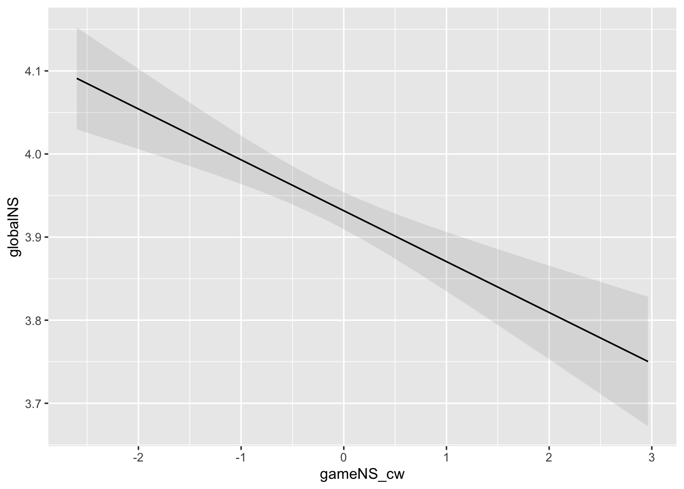

3.2 H2. Situational need satisfaction is positively associated with the likelihood of playing in the period after survey completion (H2a), while global need frustration is negatively associated (H2b)

Experiences of need satisfaction during a particular gaming session lead players to update expectations for future experiences with the current game, similar games, and gaming as a whole, such that greater need satisfaction leads to higher expectations for future need satisfaction. Under BANG, need-related outcome expectations are conceptually similar to intrinsic motivation, and the behavioral product of these expectations is therefore greater behavioral engagement.

Thus, the model attempts to evaluate whether experiencing high game-level need satisfaction in one’s most recent session is linked with a higher likelihood of playing games again in the 24-hour period after the survey.

Another factor that might increase the likelihood that someone (re)turns to gaming is global need frustration. SDT predicts that (global) need frustration results in compensatory behavior—people attempt to replenish needs that are not being met by altering their behavior. The dense need satisfaction offered by games constitute one way for people to compensate. BANG operationalizes this compensatory play in via intrinsic motivation. Frustrated needs in one’s life in general make opportunities to fulfill those needs more salient, which—all else equal—manifests phenomenologically as an increased energy towards those activities. Given this, we predict: Global need frustration is associated with higher likelihood of playing in the 24-hour period after survey completion (H9 in BANG)

As they share an outcome variable, we model these together. We model these with a multilevel within-between logistic regression, where in-game need satisfaction and global need frustration (each within- and between-person centered; gameNS_cw, gameNS_cb, globalNF_cw, globalNF_cb) predict playedAfterSurvey, a binary variable indicating whether any play happened in the 24-hour period after diary survey completion.

As before, we include an AR(1) term to account for the fact that likelihood of play might be autocorrelated (if, e.g., people tend to get on a roll and play multiple days in a row).

h2mod <- glmmTMB(
  playedLaterAny ~ gameNS_cw + gameNS_cb + globalNF_cw + globalNF_cb +
    (1 + gameNS_cw + globalNF_cw | pid) + ar1(day + 0 | pid),
  data = dat,
  family = binomial(link = "logit"),
  dispformula = ~1,
  ziformula = ~0
)

summary(h2mod)

 Family: binomial  ( logit )
Formula:          
playedLaterAny ~ gameNS_cw + gameNS_cb + globalNF_cw + globalNF_cb +  
    (1 + gameNS_cw + globalNF_cw | pid) + ar1(day + 0 | pid)
Data: dat

     AIC      BIC   logLik deviance df.resid 
      NA       NA       NA       NA     6956 

Random effects:

Conditional model:
 Groups Name        Variance   Std.Dev.   Corr                            
 pid    (Intercept)  1.041e+00  1.020e+00                                 
        gameNS_cw    5.545e-04  2.355e-02 -1.00                           
        globalNF_cw  1.887e-03  4.344e-02 -1.00       1.00                
 pid.1  day1        3.123e-299 5.588e-150 1.00 (ar1) 1.00 (ar1) 1.00 (ar1)
Number of obs: 6969, groups:  pid, 973

Conditional model:
            Estimate Std. Error z value Pr(>|z|)    
(Intercept) -0.19893    0.04339  -4.584 4.56e-06 ***
gameNS_cw    0.01047    0.02529   0.414   0.6790    
gameNS_cb   -0.28593    0.11771  -2.429   0.0151 *  
globalNF_cw -0.03674    0.03942  -0.932   0.3514    
globalNF_cb  0.02889    0.22881   0.126   0.8995    
---
Signif. codes:  0 '***' 0.001 '**' 0.01 '*' 0.05 '.' 0.1 ' ' 1

plot_predictions(h2mod, condition = "globalNF_cw", vcov = TRUE)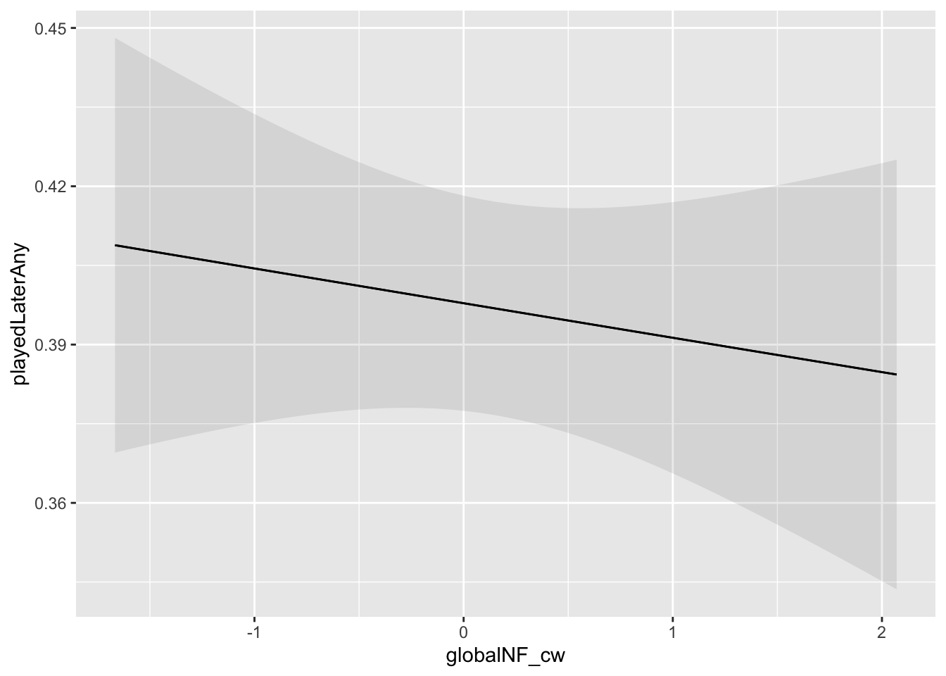

plot_predictions(h2mod, condition = "gameNS_cw", vcov = TRUE)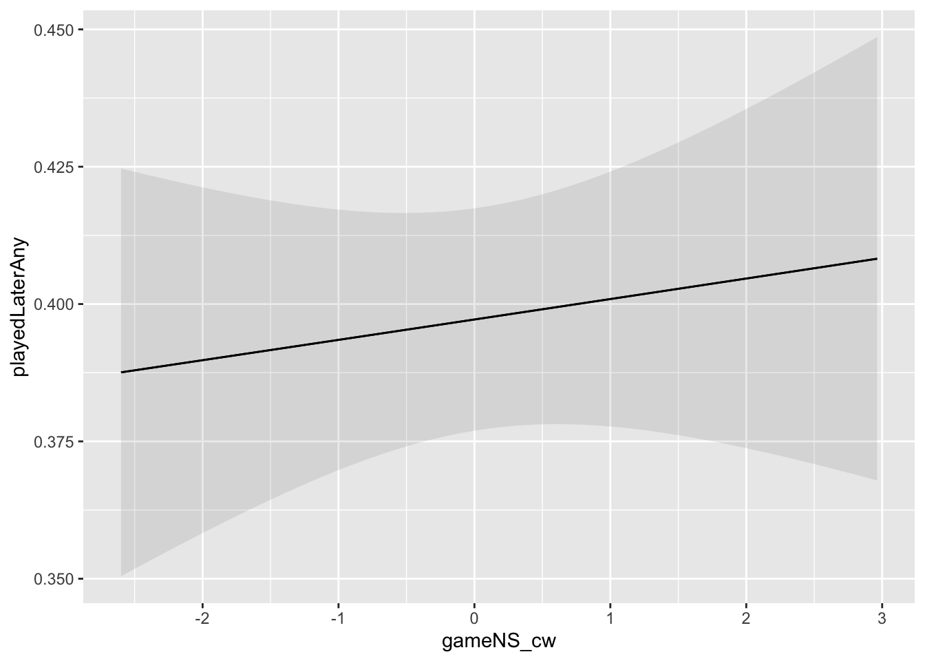

3.3 H3. When gaming displaces a core life domain (work/school, social engagements, sleep/eating/fitness, or caretaking), global need satisfaction will be lower (H5 in BANG)

We don’t have temporal precedence here (the need satisfaction measure refers to the day as a whole), and have very little ability to define and adjust for confounds, so this is a very weak test of the displacement hypothesis—but the first of its kind, as far as I know.

Briefly, I’m just interested in whether gaming sessions that displace a core life domain—work/school, social engagements, sleep/eating/fitness, or caretaking—are associated with lower global need satisfaction. displacedCoreActivity is a binary variable; participants write in a free text response what they most likely would have done instead of their most recent gaming session, and these are classified into core/noncore domains.

We use a multilevel linear regression to determine whether displacing a core activity is likely to co-occur with a person differing from their typical level of global need satisfaction (globalNS).

h3mod <- glmmTMB(globalNS ~ displacedCoreDomain + (1 + displacedCoreDomain | pid) + ar1(day + 0 | pid),
  data = dat
)
plot_predictions(h3mod, condition = "displacedCoreDomain", vcov = TRUE)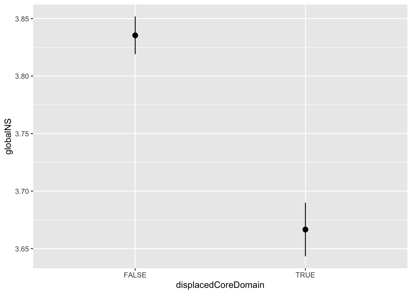

3.4 Precision Analysis

The above models are fit to simulated data which mirrors the structure of the true data, but lacks control over the distribution and relationships between the particular variables used in this study. To provide rough indications of the estimated precision of Study 1 tests, here we simulate a dataset with a known relationship between need satisfaction in games and need satisfaction in daily life, and then fit H1 as above (selecting just one hypothesis for detailed inspection to illustrate).

# sim parameters
n_pid <- 1000  
n_days <- 21
beta_0 <- 2.0  # global intercept
beta_cw <- 0.1  # global slope for within-person 
beta_cb <- 0.1  # global slope for between-person 
sigma_cw <- .5
sigma_intercept <- 1.0  # Random intercept SD
sigma_slope <- 0.5  # Random slope SD
sigma_residual <- 1  # Residual SD
rho <- 0.2  # AR(1) autocorrelation coefficient

sim_s1 <- dat |> 
  group_by(pid) |>
  mutate(
    random_intercept = rnorm(1, mean = 0, sd = sigma_intercept),
    random_slope = rnorm(1, mean = 0, sd = sigma_slope),
    gameNS_cb = rnorm(1)
  ) |> 
  ungroup() |> 
  mutate(
    gameNS_cw = rnorm(n(), mean = 0, sd = sigma_cw),
  )

# Generate AR(1) errors for each individual
sim_s1$residual <- unlist(lapply(1:n_pid, function(i) {
  arima.sim(n = n_days, model = list(ar = rho), sd = sigma_residual)
}))

# Generate the response variable based on the model
sim_s1 <- sim_s1 |> 
  mutate(globalNS = beta_0 + random_intercept + (beta_cw + random_slope)*gameNS_cw + beta_cb * gameNS_cb + residual)

h1mod <- glmmTMB(globalNS ~ gameNS_cw + gameNS_cb + (1 + gameNS_cw| pid) + ar1(as.factor(day) + 0 | pid),
  data = sim_s1
)

summary(h1mod)

 Family: gaussian  ( identity )
Formula:          
globalNS ~ gameNS_cw + gameNS_cb + (1 + gameNS_cw | pid) + ar1(as.factor(day) +  
    0 | pid)
Data: sim_s1

     AIC      BIC   logLik deviance df.resid 
 62999.8  63071.4 -31490.9  62981.8    20991 

Random effects:

Conditional model:
 Groups   Name            Variance Std.Dev. Corr                 
 pid      (Intercept)     0.9922   0.9961                        
          gameNS_cw       0.2218   0.4710   -0.02                
 pid.1    as.factor(day)1 0.8922   0.9446   0.23 (ar1) 0.23 (ar1)
 Residual                 0.1449   0.3807                        
Number of obs: 21000, groups:  pid, 1000

Dispersion estimate for gaussian family (sigma^2): 0.145 

Conditional model:
            Estimate Std. Error z value Pr(>|z|)    
(Intercept)  1.97178    0.03266   60.37  < 2e-16 ***
gameNS_cw    0.11351    0.02058    5.52 3.47e-08 ***
gameNS_cb    0.07032    0.03303    2.13   0.0332 *  
---
Signif. codes:  0 '***' 0.001 '**' 0.01 '*' 0.05 '.' 0.1 ' ' 1

plot_predictions(h1mod, condition = "gameNS_cw", vcov = TRUE, re.form = NA) +
  ylim(1, 5)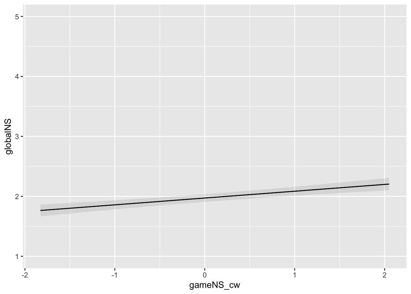

confint(h1mod)[2,3] - confint(h1mod)[2,2]

[1] -0.04033081