4 Main analysis

This document contains the main analyses presented in the manuscript.

We first load the required R packages.

library(knitr)
library(scales)
library(DT)
library(kableExtra)
library(ggpp)
library(bayestestR)
library(brms)
library(ragg)
library(here)
library(ggtext)
library(ggstance)
library(ggdist)
library(memoise)
library(cachem)
library(patchwork)
library(lavaan)
library(multidplyr)
library(tidyverse)
library(tidybayes)
library(janitor)
cd <- cache_disk("memoise")

Define plotting, table, and parallel processing options.

# parallel computations
MAX_CORES <- as.numeric(Sys.getenv("MAX_CORES"))
if (is.na(MAX_CORES)) MAX_CORES <- parallel::detectCores(logical = FALSE)
cluster <- new_cluster(MAX_CORES)

# load packages on clusters
cluster_library(cluster, c("dplyr", "lavaan"))

# MCMC settings
options(mc.cores = 1)
if (require("cmdstanr")) options(brms.backend = "cmdstanr")

# Save outputs here
dir.create("models", FALSE)

# Functions in R/
source(here("R", "meta-analysis-helpers.R"))

We analyse the data cleaned previously.

data_path <- here("Data", "cleaned_data.rds")
if (file.exists(data_path)) {
  d <- read_rds(file = data_path)
} else {
  stop(str_glue("{data_path} doesn't exist, run `01-clean.Rmd` to create it."))
}

# Make wave a nicely labelled factor
d <- d %>%
  mutate(Wave = factor(wid, levels = 1:3, labels = paste0("Wave ", 1:3)))

# Rename game to fit titles in plots
d <- d %>% 
  mutate(Game = if_else(Game == "Gran Turismo Sport", "GT Sport", Game))

For all analyses, game time indicates average number of hours per day. The telemetry indicates total hours in the two week window, so we divide that by 14 to talk about average hours per day.

d <- d %>%
  mutate(
    Hours = Hours / 14,
    hours_est = hours_est / 14
  )

4.1 Variables over time

Hours played per week is cut at a reasonable value for the figures:

d %>%
  mutate(Hours_over_3 = Hours > 3) %>%
  tabyl(Hours_over_3) %>%
  adorn_pct_formatting() %>% 
  kbl(caption = "Table of hours excluded from figure") %>% 
  kable_classic(full_width = FALSE, html_font = Font)

Table 3.3: Table of hours excluded from figure

Hours_over_3	n	percent	valid_percent
FALSE	113595	97.3%	97.4%
TRUE	3075	2.6%	2.6%
NA	100	0.1%

tmp <- d %>%
  select(
    Game, Wave, pid,
    Hours, Affect, `Life satisfaction`,
    Intrinsic, Extrinsic
  ) %>%
  pivot_longer(Hours:Extrinsic) %>%
  drop_na(value) %>%
  filter(!(name == "Hours" & value > 3)) %>%
  mutate(name = if_else(name == "Hours", "Hours / day", name)) %>% 
  mutate(name = fct_inorder(name))
tmp %>%
  ggplot(
    aes(
      Wave,
      value
    )
  ) +
  scale_x_discrete(labels = 1:3, expand = expansion(c(0.1, .1))) +
  scale_y_continuous(
    "Value",
    breaks = pretty_breaks(),
    expand = expansion(.025)
  ) +
  geom_blank() +
  stat_halfeye(
    height = .02,
    normalize = "panels",
    slab_color = col1,
    slab_fill = alpha(col1, 0.3),
    slab_size = 0.5,
    adjust = 1.1,
    point_interval = NULL,
    show.legend = FALSE
  ) +
  stat_summary(
    fun.data = mean_cl_normal,
    fatten = 1.25
  ) +
  stat_summary(
    fun = mean,
    geom = "line",
    size = .33,
    group = 1
  ) +
  facet_grid(name ~ Game, scales = "free_y") +
  theme(
    legend.position = "none"
  )

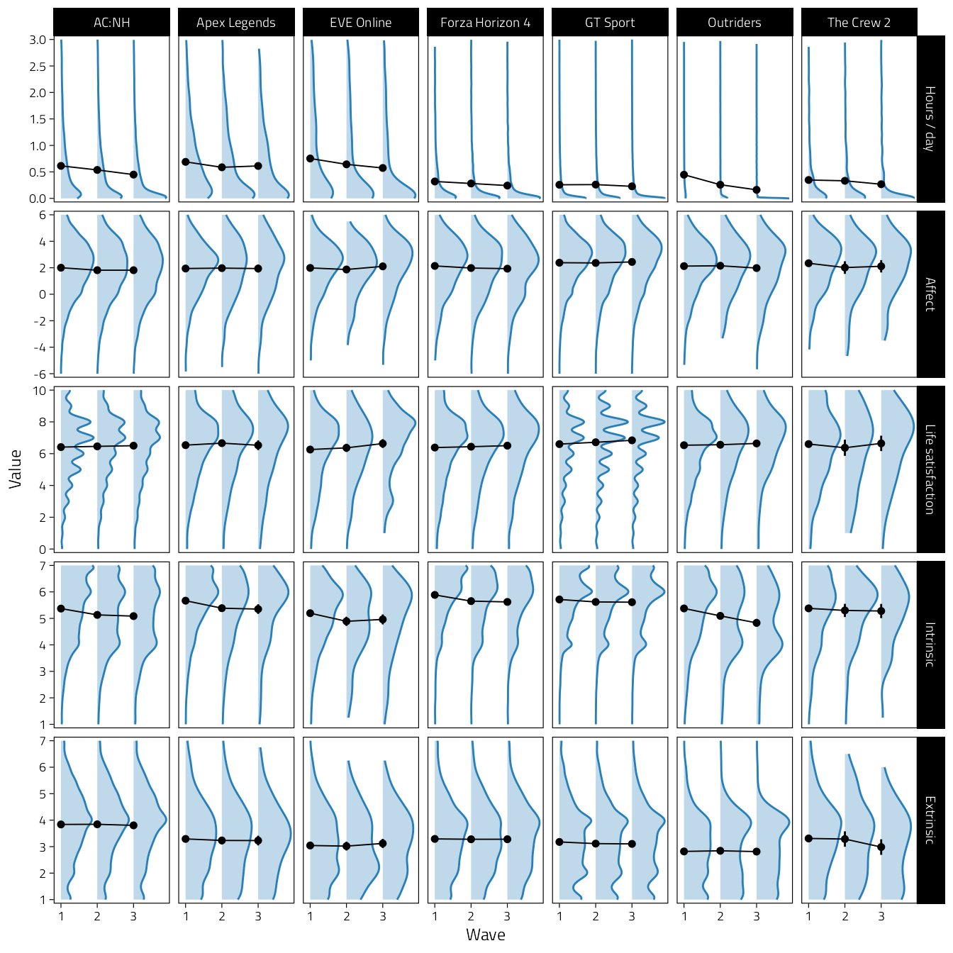
Figure 4.1: Density plots of key variables over time.

Then take a look at a simple model of change over time for each variable. Note that we can’t use varying slopes with lmer because there’s not enough data, so just random intercepts for players.

library(lme4)
library(broom.mixed)
path <- "models/parameters_change_over_time.rds"
if (!file.exists(path)) {
  parameters_change_over_time <- d %>%
    select(
      Game, pid, wid,
      Hours, Intrinsic, Extrinsic,
      Affect, `Life satisfaction`
    ) %>%
    # Put intercept at first wave
    mutate(Wave = wid - 1) %>%
    pivot_longer(Hours:`Life satisfaction`, names_to = "Variable") %>%
    group_by(Variable) %>%
    summarise(
      lmer(value ~ Wave + (1 | pid) + (1 + Wave | Game), data = cur_data()) %>%
        tidy(., "fixed", conf.int = TRUE)
    )
  saveRDS(parameters_change_over_time, path)
} else {parameters_change_over_time <- readRDS(path)}

parameters_change_over_time %>%
  mutate(across(where(is.numeric), ~ format(round(.x, 2), nsmall = 2))) %>%
  mutate(Result = str_glue("{estimate}, 95%CI [{conf.low}, {conf.high}]")) %>%
  select(Variable, term, Result) %>%
  pivot_wider(names_from = term, values_from = Result) %>% 
  kbl(caption = "Change over time parameter estimates") %>% 
  kable_classic(full_width = FALSE, html_font = Font)

Table 4.1: Change over time parameter estimates

Variable	(Intercept)	Wave
Affect	2.12, 95%CI [ 2.00, 2.24]	-0.05, 95%CI [-0.10, -0.01]
Extrinsic	3.25, 95%CI [ 3.02, 3.48]	-0.01, 95%CI [-0.03, 0.01]
Hours	0.69, 95%CI [ 0.39, 1.00]	-0.09, 95%CI [-0.15, -0.04]
Intrinsic	5.51, 95%CI [ 5.33, 5.69]	-0.18, 95%CI [-0.23, -0.13]
Life satisfaction	6.47, 95%CI [6.40, 6.55]	0.05, 95%CI [0.03, 0.08]

4.2 Simple correlation

Before more informative modelling, we estimate simple bivariate regressions between the key variables.

tmp <- d %>% 
  arrange(pid, wid) %>% 
  group_by(pid) %>% 
  mutate(h1 = lag(Hours))

fit <- lmer(Affect ~ h1 + (1 | pid) + (h1 | Game), data = tmp)
summary(fit)

## Linear mixed model fit by REML ['lmerMod']
## Formula: Affect ~ h1 + (1 | pid) + (h1 | Game)
##    Data: tmp
## 
## REML criterion at convergence: 101413.9
## 
## Scaled residuals: 
##     Min      1Q  Median      3Q     Max 
## -4.4954 -0.3566  0.0485  0.3947  3.9020 
## 
## Random effects:
##  Groups   Name        Variance Std.Dev. Corr 
##  pid      (Intercept) 3.391653 1.84164       
##  Game     (Intercept) 0.045830 0.21408       
##           h1          0.001198 0.03461  -1.00
##  Residual             0.992279 0.99613       
## Number of obs: 25181, groups:  pid, 17197; Game, 7
## 
## Fixed effects:
##             Estimate Std. Error t value
## (Intercept)  1.97604    0.08972  22.024
## h1           0.07184    0.02063   3.483
## 
## Correlation of Fixed Effects:
##    (Intr)
## h1 -0.750
## optimizer (nloptwrap) convergence code: 0 (OK)
## boundary (singular) fit: see ?isSingular

d %>%
  select(
    Game, pid, wid, Wave,
    Hours, hours_est, Intrinsic, Extrinsic,
    Affect, `Life satisfaction`
  ) %>%
  pivot_longer(
    c(Affect, `Life satisfaction`),
    names_to = "Outcome", values_to = "Outcome_value"
  ) %>%
  pivot_longer(
    c(Hours, hours_est, Intrinsic, Extrinsic),
    names_to = "Predictor", values_to = "Predictor_value"
  ) %>%
  group_by(Game, Outcome, Predictor, Wave) %>%
  summarise(
    tidy(
      lm(
        Outcome_value ~ Predictor_value, 
        data = cur_data()
      ), 
      conf.int = TRUE
    ),
  ) %>%
  filter(term != "(Intercept)") %>%
  ggplot(aes(estimate, Game, col = Wave)) +
  geom_vline(xintercept = 0, lty = 2, size = .25) +
  scale_x_continuous(
    "Bivariate regression coefficient (95%CI)",
    breaks = pretty_breaks()
  ) +
  geom_pointrangeh(
    aes(xmin = conf.low, xmax = conf.high),
    size = .4,
    position = position_dodge2v(.35)
  ) +
  facet_grid(Outcome ~ Predictor) +
  theme(
    legend.position = "bottom",
    axis.title.y = element_blank()
  )

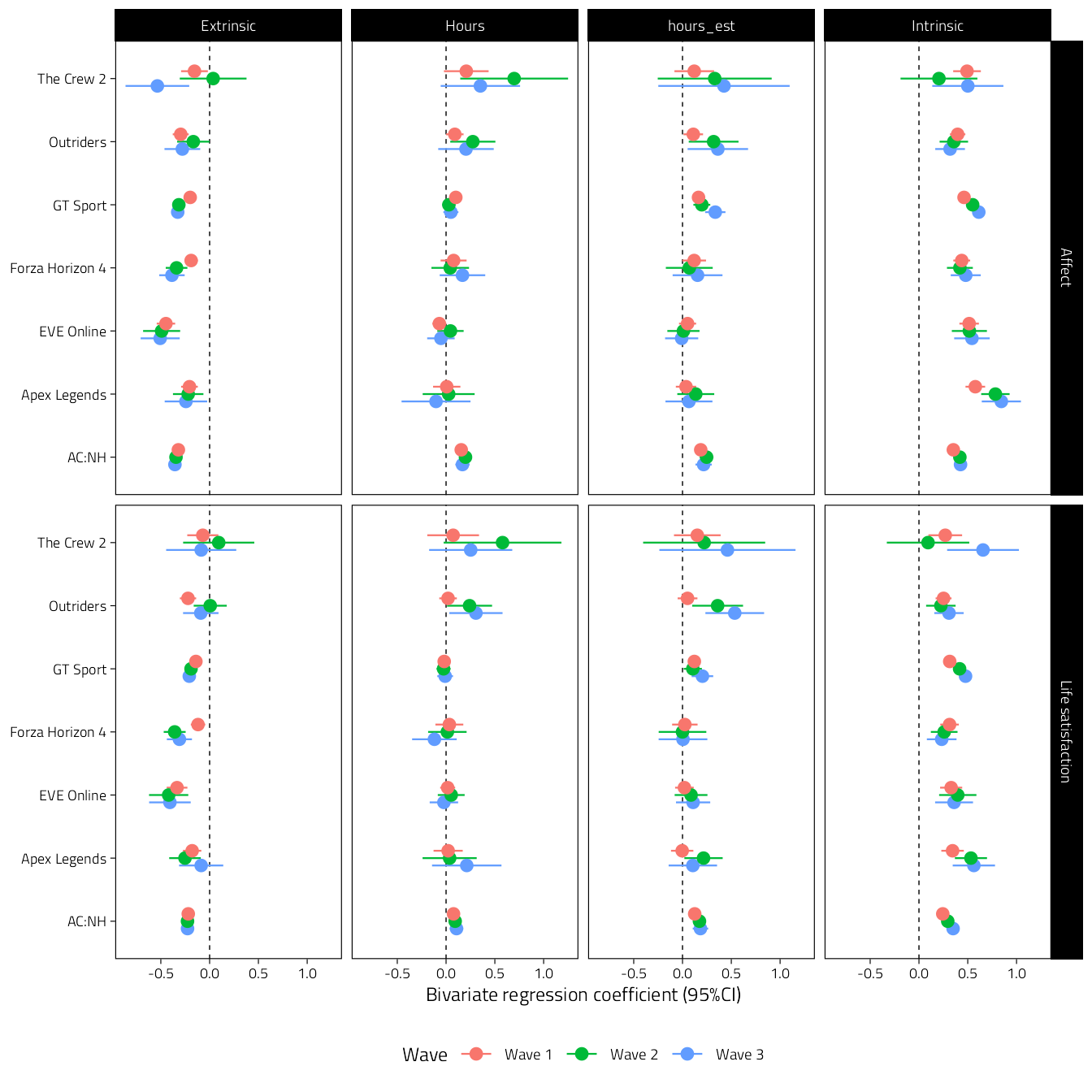
Figure 4.2: Unstandardised bivariate regression coefficients of models predicting well-being. Columns indicate predictors, and the two rows are the different well-being outcome variables.

4.3 RICLPM

Wrangle data to a format where lavaan model is easier to map to variable pairs: Wide format with different rows for outcomes (well-being) and predictors (hours, needs, motivations).

d_riclpm_long <- d %>%
  select(
    Game, pid, wid,
    Hours, hours_est,
    Intrinsic, Extrinsic,
    Affect, `Life satisfaction`, AN, AP
  ) %>%
  # Long format on well-being scores (outcomes)
  pivot_longer(
    c(Affect, `Life satisfaction`, AN, AP),
    names_to = "y_var", values_to = "y"
  ) %>%
  # Long format on other variables (predictors)
  pivot_longer(
    c(Hours, hours_est, Intrinsic, Extrinsic),
    names_to = "x_var", values_to = "x"
  )
d_riclpm_wide <- d_riclpm_long %>%
  pivot_wider(names_from = wid, values_from = c(x, y), names_sep = "")
write_rds(d_riclpm_wide, here("Temp", "d_riclpm_wide.rds"))

4.3.1 Cross-lagged scatterplots

Order <- tibble(
  y_var = rep(c("Affect", "Life satisfaction"), each = 2),
  wid = c(2, 3, 2, 3),
  Panel = c(
    "Affect[plain('[Wave 2]')]",
    "Affect[plain('[Wave 3]')]",
    "LS[plain('[Wave 2]')]",
    "LS[plain('[Wave 3]')]"
  ),
  Panel_label = fct_inorder(Panel)
)

d_riclpm_plots <- d_riclpm_long %>%
  # Don't show AN and AP
  filter(!(y_var %in% c("AN", "AP"))) %>% 
  # Take out hours per day over 3 for these plots
  mutate(x = if_else(str_detect(x_var, "ours") & x > 3, NaN, x)) %>%
  arrange(Game, pid, x_var, wid) %>%
  group_by(Game, pid, x_var, y_var) %>%
  mutate(lag_x = lag(x)) %>%
  left_join(Order) %>%
  ungroup() %>%
  filter(wid > 1)

d_riclpm_plots %>%
  filter(x_var == "Hours") %>%
  ggplot(aes(lag_x, y)) +
  scale_x_continuous(
    "Hours played per day at previous wave",
    breaks = pretty_breaks(3)
  ) +
  scale_y_continuous(
    "Well-being at current wave",
    breaks = pretty_breaks()
  ) +
  geom_point(size = .2, alpha = .2, shape = 1, col = col1) +
  geom_smooth(
    method = "gam", size = .4,
    color = "black",
    alpha = .33, show.legend = FALSE
  ) +
  facet_grid(
    Panel_label ~ Game,
    scales = "free_y",
    labeller = labeller(.rows = label_parsed)
  ) +
  theme(
    aspect.ratio = 1,
    panel.grid = element_blank()
  )

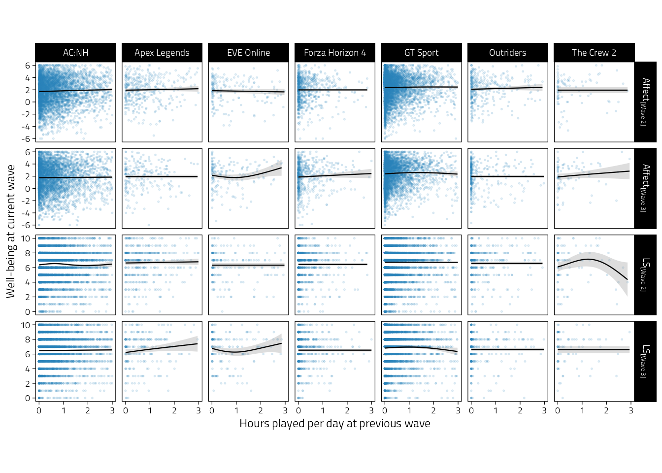
Figure 4.3: Scatterplots of well-being (rows indicate variables and waves) on average hours played per day during the previous wave. Regression lines are GAM fitted lines and 95%CIs.

# Plots with other predictors
p_tmp_0 <- last_plot() %+%
  filter(d_riclpm_plots, x_var == "hours_est") +
  scale_x_continuous(
    "Estimated hours played per day at previous wave",
    breaks = 0:3
  )
p_tmp_0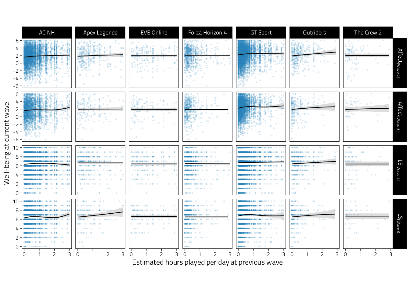

Figure 4.4: Scatterplots of well-being (rows indicate variables and waves) on estimated average hours played per day during the previous wave. Regression lines are GAM fitted lines and 95%CIs.

p_tmp_1 <- last_plot() %+%
  filter(d_riclpm_plots, x_var == "Intrinsic") +
  scale_x_continuous(
    "Intrinsic motivation at previous wave",
    breaks = pretty_breaks()
  )
p_tmp_1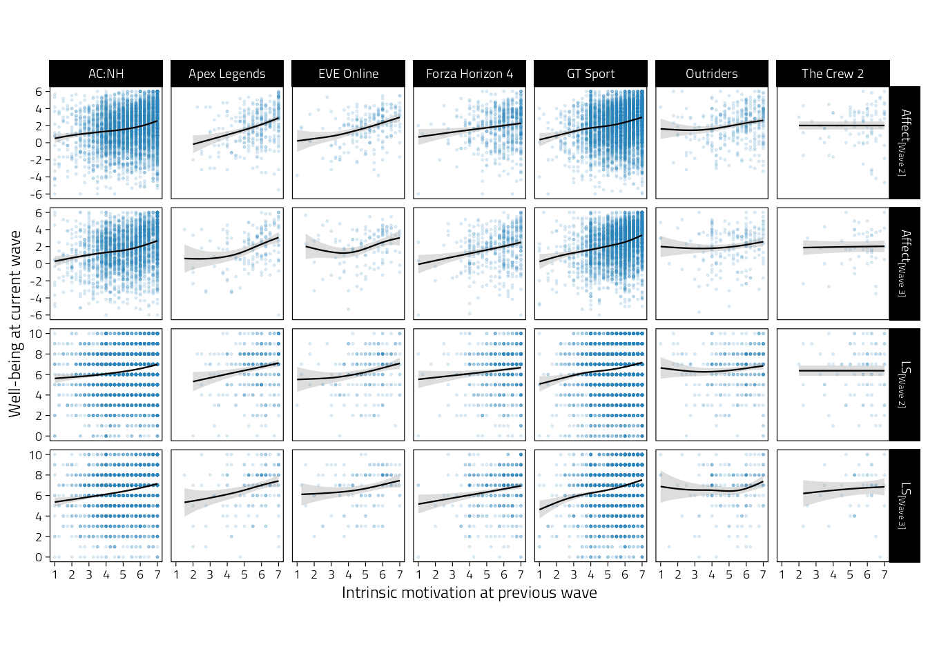

Figure 4.5: Scatterplots of well-being (rows indicate variables and waves) on intrinsic motivation during the previous wave. Regression lines are GAM fitted lines and 95%CIs.

p_tmp_2 <- last_plot() %+%
  filter(d_riclpm_plots, x_var == "Extrinsic") +
  scale_x_continuous(
    "Extrinsic motivation at previous wave",
    breaks = pretty_breaks()
  )
p_tmp_2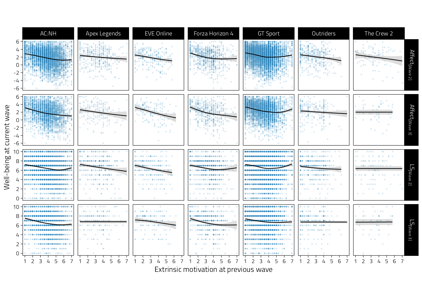

Figure 4.6: Scatterplots of well-being (rows indicate variables and waves) on extrinsic motivation during the previous wave. Regression lines are GAM fitted lines and 95%CIs.

p_tmp_1 / p_tmp_2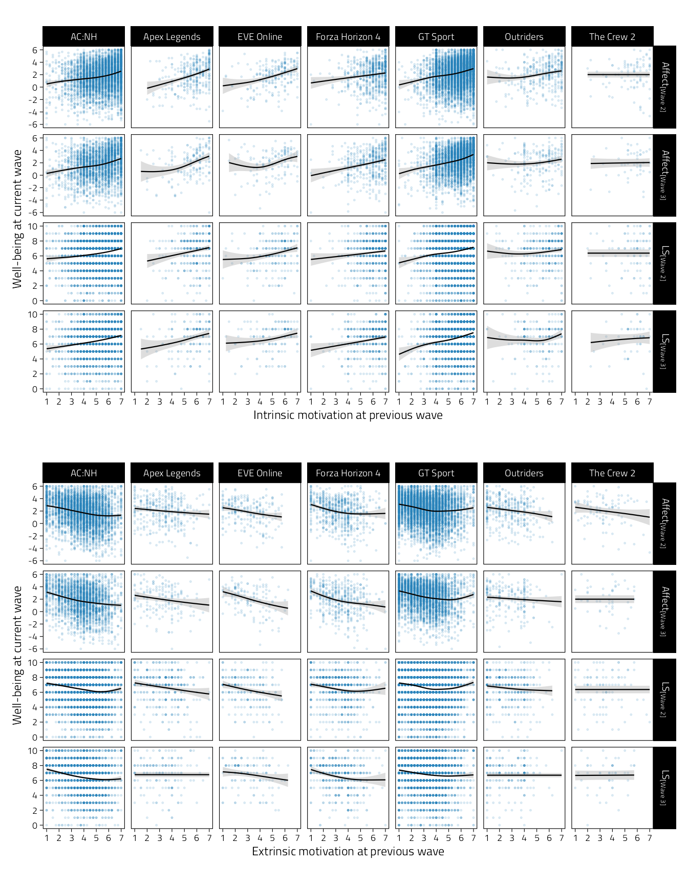

Figure 4.7: Scatterplots of well-being (rows indicate variables and waves) on intrinsic and extrinsic motivation during the previous wave. Regression lines are GAM fitted lines and 95%CIs.

4.3.2 Fit models

First fit RICLPM to all data. Separately to the two well-being outcomes, and each predictor (hours, subjective scales). Constrain (cross)lagged parameters

Syntax based on https://jeroendmulder.github.io/RI-CLPM/lavaan.html

riclpm_1 <- "
  # Create between components (random intercepts)
  RIx =~ 1*x1 + 1*x2 + 1*x3
  RIy =~ 1*y1 + 1*y2 + 1*y3

  # Create within-person centered variables
  wx1 =~ 1*x1
  wx2 =~ 1*x2
  wx3 =~ 1*x3
  wy1 =~ 1*y1
  wy2 =~ 1*y2
  wy3 =~ 1*y3

  # Estimate the lagged effects between the within-person centered variables (constrained).
  wx2 ~ bx*wx1 + gx*wy1
  wy2 ~ gy*wx1 + by*wy1
  wx3 ~ bx*wx2 + gx*wy2
  wy3 ~ gy*wx2 + by*wy2

  # Estimate the covariance between the within-person centered
  # variables at the first wave.
  wx1 ~~ wy1 # Covariance

  # Estimate the covariances between the residuals of the
  # within-person centered variables (the innovations).
  wx2 ~~ wy2
  wx3 ~~ wy3

  # Estimate the variance and covariance of the random intercepts.
  RIx ~~ RIx
  RIy ~~ RIy
  RIx ~~ RIy

  # Estimate the (residual) variance of the within-person centered variables.
  wx1 ~~ wx1 # Variances
  wy1 ~~ wy1
  wx2 ~~ wx2 # Residual variances
  wy2 ~~ wy2
  wx3 ~~ wx3
  wy3 ~~ wy3
"

# This is the same but was suggested to not include autoregressions
riclpm_2 <- [1109 chars quoted with '"']

cluster_library(cluster, "purrr")
cluster_copy(cluster, c("riclpm_1", "riclpm_2"))
path <- "models/riclpm-pooled.rds"
if (!file.exists(path)) {
  fit_riclpm_all <- d_riclpm_wide %>%
    group_by(y_var, x_var) %>%
    nest() %>% 
    crossing(
      nesting(
        lvn = c(riclpm_1, riclpm_2), 
        model = c("1", "2")
      )
    ) %>% 
    partition(cluster) %>%
    mutate(
      fit = map2(
        data, lvn,
        ~lavaan(
          .y,
          data = .x,
          missing = "ml",
          meanstructure = TRUE,
          int.ov.free = TRUE
        )
      )
    ) %>%
    collect() %>% 
    ungroup() %>% 
    select(-data, -lvn)
  saveRDS(fit_riclpm_all, path)
} else {fit_riclpm_all <- readRDS(path)}

Fit the above model separately to each game.

path <- "models/riclpm-games.rds"
if (!file.exists(path)) {
  fit_riclpm_games <- d_riclpm_wide %>%
    group_by(y_var, x_var, Game) %>%
    nest() %>% 
    crossing(
      nesting(
        lvn = c(riclpm_1, riclpm_2), 
        model = c("1", "2")
      )
    ) %>% 
    partition(cluster) %>%
    mutate(
      fit = map2(
        data, lvn,
        ~lavaan(
          .y,
          data = .x,
          missing = "ml",
          meanstructure = TRUE,
          int.ov.free = TRUE
        )
      )
    ) %>%
    collect() %>% 
    ungroup() %>% 
    select(-data, -lvn)
  saveRDS(fit_riclpm_games, path)
} else {fit_riclpm_games <- readRDS(path)}

get_lavaan_pars <- function(x) {
  bind_rows(
    parameterestimates(x) %>%
      mutate(Type = "Unstandardized"),
    standardizedsolution(x) %>%
      rename(est = est.std) %>%
      mutate(Type = "Standardized")
  ) %>%
    as_tibble() %>%
    unite("Parameter", c(lhs, op, rhs), sep = " ", remove = FALSE)
}

pars_riclpm <- bind_rows(
  "Pooled" = fit_riclpm_all,
  "Independent" = fit_riclpm_games,
  .id = "Fit"
) %>% 
  mutate(pars = map(fit, get_lavaan_pars)) %>%
  select(-fit)

# Take only parameters of interest
pars_riclpm <- pars_riclpm %>% 
  unnest(pars) %>% 
    filter(
    (str_detect(Parameter, " ~ ") & !str_detect(Parameter, "3")) |
      Parameter %in% c("RIx ~~ RIy", "wx1 ~~ wy1", "wx2 ~~ wy2", "wx3 ~~ wy3")
  ) %>% 
  select(-c(lhs:label, z))

pars_riclpm %>%
  filter(Fit == "Pooled", model == "1") %>% 
  filter(
    str_detect(Parameter, " ~ "),
    Type == "Unstandardized"
  ) %>%
  mutate(across(where(is.numeric), ~ format(round(.x, 2), nsmall = 2))) %>%
  mutate(Result = str_glue("{est}, [{ci.lower}, {ci.upper}]")) %>%
  select(y_var, x_var, Parameter, Result) %>%
  pivot_wider(names_from = Parameter, values_from = Result) %>%
  arrange(y_var, x_var) %>% 
  kbl(
    caption = "RICLPM regression parameters from pooled model."
  ) %>% 
  kable_classic(full_width = FALSE, html_font = Font)

Table 4.2: RICLPM regression parameters from pooled model.

y_var	x_var	wx2 ~ wx1	wx2 ~ wy1	wy2 ~ wx1	wy2 ~ wy1
Affect	Extrinsic	0.22, [ 0.18, 0.27]	-0.06, [-0.08, -0.04]	-0.12, [-0.17, -0.07]	0.35, [ 0.32, 0.39]
Affect	Hours	0.47, [ 0.46, 0.49]	0.01, [ 0.00, 0.01]	-0.02, [-0.07, 0.03]	0.37, [ 0.34, 0.41]
Affect	hours_est	0.17, [ 0.14, 0.20]	0.01, [ 0.00, 0.02]	-0.03, [-0.09, 0.03]	0.37, [ 0.34, 0.41]
Affect	Intrinsic	0.35, [ 0.32, 0.39]	0.07, [ 0.06, 0.09]	0.14, [ 0.09, 0.19]	0.36, [ 0.32, 0.39]
AN	Extrinsic	0.23, [ 0.18, 0.28]	0.08, [ 0.04, 0.12]	0.08, [ 0.05, 0.11]	0.26, [ 0.22, 0.30]
AN	Hours	0.47, [ 0.46, 0.49]	-0.01, [-0.02, 0.00]	-0.01, [-0.04, 0.03]	0.28, [ 0.24, 0.32]
AN	hours_est	0.17, [ 0.14, 0.21]	-0.02, [-0.04, 0.01]	0.02, [-0.02, 0.05]	0.28, [ 0.24, 0.32]
AN	Intrinsic	0.37, [ 0.33, 0.40]	-0.11, [-0.14, -0.08]	-0.08, [-0.11, -0.05]	0.28, [ 0.24, 0.32]
AP	Extrinsic	0.23, [ 0.18, 0.28]	-0.08, [-0.11, -0.04]	-0.05, [-0.08, -0.02]	0.30, [ 0.27, 0.34]
AP	Hours	0.47, [ 0.46, 0.49]	0.01, [ 0.00, 0.02]	-0.02, [-0.05, 0.02]	0.31, [ 0.27, 0.35]
AP	hours_est	0.17, [ 0.14, 0.20]	0.01, [-0.01, 0.03]	-0.01, [-0.05, 0.03]	0.31, [ 0.27, 0.35]
AP	Intrinsic	0.36, [ 0.33, 0.40]	0.10, [ 0.07, 0.13]	0.09, [ 0.06, 0.12]	0.30, [ 0.26, 0.33]
Life satisfaction	Extrinsic	0.23, [ 0.18, 0.28]	-0.02, [-0.04, 0.00]	-0.07, [-0.14, 0.00]	0.18, [ 0.14, 0.22]
Life satisfaction	Hours	0.48, [ 0.46, 0.49]	0.00, [-0.01, 0.00]	-0.06, [-0.12, 0.01]	0.18, [ 0.14, 0.22]
Life satisfaction	hours_est	0.17, [ 0.14, 0.21]	0.01, [ 0.00, 0.02]	0.03, [-0.05, 0.11]	0.18, [ 0.14, 0.22]
Life satisfaction	Intrinsic	0.38, [ 0.34, 0.41]	0.04, [ 0.02, 0.05]	0.18, [ 0.12, 0.24]	0.18, [ 0.15, 0.22]

4.3.3 Table of parameters

This table displays the lavaan estimates (game specific and pooled) for model 1 (full RICLPM) and 2 (RICLPM without autocorrelations).

# Interactive table so reader can find what they're looking for
pars_riclpm %>% 
  mutate(
    pvalue = pvalue(pvalue),
    across(c(model, x_var, y_var, Game, Parameter, Type, Fit), factor),
    across(where(is.numeric), ~format(round(.x, 2), nsmall = 2)),
    Estimate = str_glue("{est} [{ci.lower}, {ci.upper}]")
  ) %>% 
  select(
    model, Fit, x_var, y_var, Game, Parameter, Type,
    Estimate, pvalue
  ) %>% 
  datatable(
    filter = "top",
    class = "display",
    rownames = FALSE
  ) %>% 
  formatStyle(TRUE, `font-size` = '12px')

4.4 Meta-analyses

Number of observations/participants per model

fit_riclpm_games %>%
  filter(model == 1) %>% 
  mutate(N = map_dbl(fit, nobs) %>% comma()) %>%
  select(-fit, -model) %>%
  pivot_wider(
    names_from = x_var,
    values_from = N,
    names_glue = "{x_var} {.value}"
  ) %>%
  rename(Outcome = y_var) %>%
  arrange(Outcome, Game) %>%
  kbl(caption = "Sample sizes per RICLPM") %>% 
  kable_classic(full_width = FALSE, html_font = Font)

Table 4.3: Sample sizes per RICLPM

Game	Outcome	Extrinsic N	Hours N	hours_est N	Intrinsic N
AC:NH	Affect	13,485.0	13,646.0	13,477.0	13,487.0
Apex Legends	Affect	1,127.0	1,158.0	1,125.0	1,127.0
EVE Online	Affect	886.0	905.0	887.0	886.0
Forza Horizon 4	Affect	1,951.0	1,981.0	1,953.0	1,951.0
GT Sport	Affect	18,964.0	19,258.0	18,975.0	18,972.0
Outriders	Affect	1,518.0	1,530.0	1,512.0	1,518.0
The Crew 2	Affect	448.0	457.0	446.0	448.0
AC:NH	AN	13,487.0	13,646.0	13,479.0	13,489.0
Apex Legends	AN	1,127.0	1,158.0	1,125.0	1,127.0
EVE Online	AN	886.0	905.0	887.0	886.0
Forza Horizon 4	AN	1,951.0	1,981.0	1,953.0	1,951.0
GT Sport	AN	18,966.0	19,258.0	18,976.0	18,973.0
Outriders	AN	1,518.0	1,530.0	1,512.0	1,518.0
The Crew 2	AN	449.0	457.0	447.0	449.0
AC:NH	AP	13,487.0	13,646.0	13,480.0	13,488.0
Apex Legends	AP	1,127.0	1,158.0	1,125.0	1,127.0
EVE Online	AP	886.0	905.0	887.0	886.0
Forza Horizon 4	AP	1,952.0	1,981.0	1,953.0	1,952.0
GT Sport	AP	18,976.0	19,258.0	18,980.0	18,983.0
Outriders	AP	1,518.0	1,530.0	1,512.0	1,518.0
The Crew 2	AP	448.0	457.0	446.0	448.0
AC:NH	Life satisfaction	13,621.0	13,646.0	13,587.0	13,621.0
Apex Legends	Life satisfaction	1,152.0	1,158.0	1,148.0	1,152.0
EVE Online	Life satisfaction	904.0	905.0	897.0	904.0
Forza Horizon 4	Life satisfaction	1,979.0	1,981.0	1,976.0	1,979.0
GT Sport	Life satisfaction	19,214.0	19,258.0	19,169.0	19,218.0
Outriders	Life satisfaction	1,526.0	1,530.0	1,519.0	1,526.0
The Crew 2	Life satisfaction	452.0	457.0	454.0	452.0

Then conduct all meta-analyses (for each model, y_var-x_var pair, parameter of interest, and type of parameter (standardized, unstandardized)) of the game-specific RICLPM parameters.

# Select variables from RICLPM parameters to data for MA
d_ma <- pars_riclpm %>%
  filter(
    Fit == "Independent",
    str_detect(Parameter, " ~ ") | 
      Parameter %in% c("wx1 ~~ wy1", "RIx ~~ RIy")
  ) %>%
  select(
    model, Type, y_var, 
    x_var, Game, Parameter, 
    est, se, ci.lower, ci.upper
  )
path <- "models/all-meta-analyses.rds"
if (!file.exists(path)) {
  cluster_copy(cluster, "get_ma_post")
  cluster_library(
    cluster, 
    c("brms", "purrr", "cmdstanr", "rstan", "bayestestR", "forcats")
    )
  fit_ma <- d_ma %>%
    mutate(
      name = str_glue("models/brm-{model}-{Type}-{y_var}-{x_var}-{Parameter}")
    ) %>% 
    group_by(model, x_var, y_var, Parameter, Type, name) %>%
    nest() %>% 
    partition(cluster) %>%
    mutate(
      # Fit model
      fit = map2(
        data, name,
        ~brm(
          bf(est | se(se) ~ 1 + (1 | Game)),
          data = .x,
          backend = "cmdstanr",
          prior = prior(student_t(7, 0, 0.25), class = "sd", group = "Game"),
          control = list(adapt_delta = .9999, max_treedepth = 15),
          iter = 15000, warmup = 10000,
          file = .y
        )
      ),
      # Table of posterior samples
      posterior = map(fit, get_ma_post),
      # Table of posterior summary
      summary = map(
        posterior,
        ~ describe_posterior(
          .x, 
          centrality = "mean", 
          ci = 0.95, 
          ci_method = "eti",
          test = "pd"
        ) %>%
          rename(Game = Parameter) %>% 
          mutate(Game = fct_relevel(Game, "Average")) %>% 
          as_tibble()
      ),
      # 
      sd = map(
        fit, 
        ~posterior_summary(.x, variable = "sd_Game__Intercept") %>% 
          as_tibble()
      )
    ) %>% 
    collect() %>%
    ungroup() %>% 
    select(-name, -fit)
  saveRDS(fit_ma, path, compress = FALSE)
} else {fit_ma <- readRDS(path)}

# Arrange for tables etc
fit_ma <- fit_ma %>% 
  mutate(
    model = factor(model, levels = 1:2, labels = c("AR", "No AR")),
    Type = factor(Type, levels = c("Unstandardized", "Standardized")),
    y_var = factor(
      y_var, levels = c("Affect", "Life satisfaction", "AN", "AP")
    ),
    x_var = factor(
      x_var, levels = c("Hours", "Intrinsic", "Extrinsic", "hours_est")
    ),
    Parameter = fct_relevel(Parameter, "wy2 ~ wx1")
  ) %>% 
  arrange(model, Type, y_var, x_var, Parameter)

4.4.1 Table of parameters

All the resulting parameters are listed in the table below.

fit_ma %>% 
  select(model:Parameter, summary) %>% 
  unnest(summary) %>% 
  mutate(
    across(where(is.numeric), ~format(round(.x, 2), nsmall = 2)),
    Estimate = str_glue("{Mean} [{CI_low}, {CI_high}]")
  ) %>% 
  select(model, Type, y_var, x_var, Parameter, Game, Estimate, pd) %>% 
  datatable(
    filter = "top",
    class = "display",
    rownames = FALSE
  ) %>% 
  formatStyle(TRUE, `font-size` = '12px')

4.4.2 Hours <-> WB

Draw a forest plot of meta-analyses with hours. First, define informative labels and correct order for them, and load a function for drawing forest plots.

# Table of nice labels in proper order
Order <- distinct(fit_ma, x_var, y_var, Parameter) %>%
  ungroup() %>%
  # Meta-analyses only for regression parameters
  filter(str_detect(Parameter, " ~ ")) %>%
  mutate(
    x_lab = case_when(
      x_var == "Hours" ~ "Play",
      x_var == "Intrinsic" ~ "Intrinsic",
      x_var == "Extrinsic" ~ "Extrinsic"
    ),
    y_lab = case_when(
      y_var == "Affect" ~ "Affect",
      y_var == "Life satisfaction" ~ "Life~satisfaction"
    ),
    Panel_label = case_when(
      Parameter == "wx2 ~ wx1" ~
        str_glue('{x_lab}[plain("[t-1]")]%->%{x_lab}[plain("[t]")]'),
      Parameter == "wy2 ~ wy1" ~
        str_glue('{y_lab}[plain("[t-1]")]%->%{y_lab}[plain("[t]")]'),
      Parameter == "wy2 ~ wx1" ~
        str_glue('{x_lab}[plain("[t-1]")]%->%{y_lab}[plain("[t]")]'),
      Parameter == "wx2 ~ wy1" ~
        str_glue('{y_lab}[plain("[t-1]")]%->%{x_lab}[plain("[t]")]')
    )
  ) %>%
  mutate(
    Parameter_order = factor(
      Parameter,
      levels = c("wy2 ~ wx1", "wx2 ~ wy1")
    )
  ) %>%
  arrange(Parameter_order, y_var) %>%
  mutate(Panel_label = fct_inorder(Panel_label))

# Only these are needed
forest_plot_data <- fit_ma %>% 
  filter(
    model == "AR", 
    Type == "Unstandardized",
    y_var %in% c("Affect", "Life satisfaction"),
    x_var %in% c("Hours", "Intrinsic", "Extrinsic"),
    Parameter %in% c("wy2 ~ wx1", "wx2 ~ wy1")
  ) %>% 
  left_join(Order) %>% 
  select(-model, -Type)

forest_plot_data %>% 
  filter(x_var == "Hours") %>% 
  forest_plot()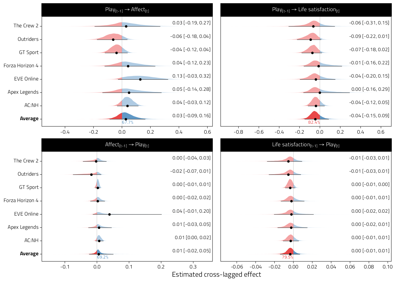

Figure 4.8: Plot

# Also see in comparison to lavaan model estimates
forest_plot_data %>% 
  filter(x_var == "Hours") %>% 
  forest_plot(lavaan = TRUE)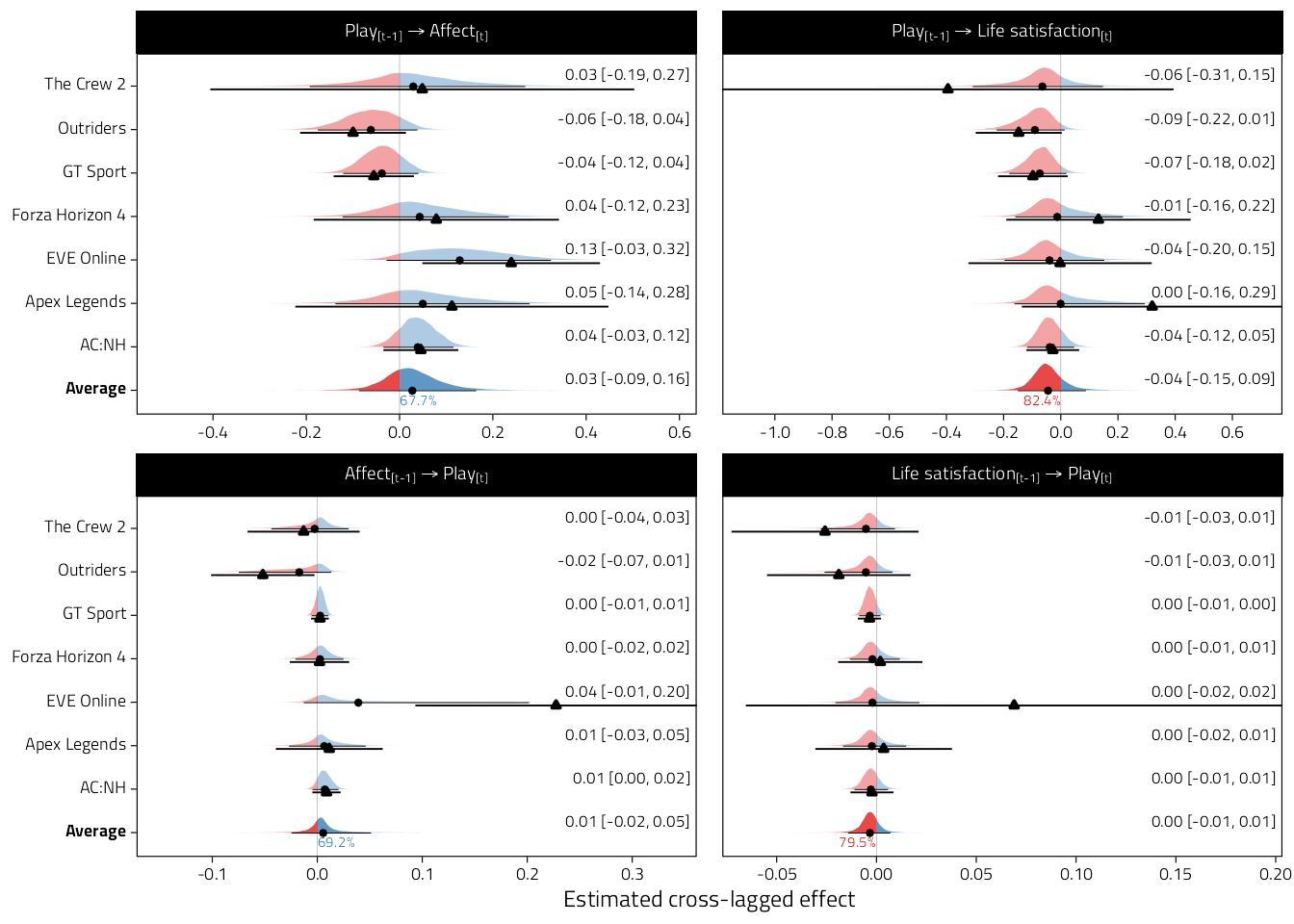

Figure 4.9: Figure as above but also displaying the underlying lavaan fits’ point estimates and 95%CIs.

4.4.3 Experiences <-> WB

a <- forest_plot_data %>% 
  filter(x_var %in% c("Intrinsic"), Parameter == "wy2 ~ wx1") %>% 
  forest_plot() +
  theme(axis.title.x = element_blank())

b <- forest_plot_data %>% 
  filter(x_var %in% c("Extrinsic"), Parameter == "wy2 ~ wx1") %>% 
  forest_plot()

a/b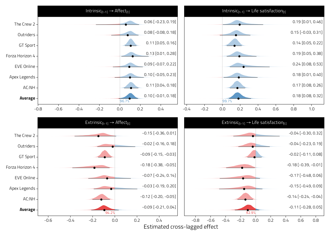

Figure 4.10: Forest plots of meta-analytic raw cross-lagged regression coefficients from models examining motivations and well-being (motivations to well-being). Shaded curves indicate approximate posterior densities, which are numerically summarised by means and 95%CIs in the right margin. Numbers below average effects indicate posterior probabilities of direction.

4.4.4 Some post-hoc calculations

The model parameters report effects of one-unit (e.g. one hour per day) changes in the predictor on the outcome. We also expand on this by first asking what is the effect of an average deviation in a predictor on the outcome. That is, for example, we calculate the average range of players’ average daily hours played, and then answer what the effect of an average player moving from their smallest to greatest amount of play would be on well-being.

# Average ranges of predictors
avg_ranges <- d %>%
  # Calculate range for everyone (returns -Inf if all values missing)
  group_by(Game, pid) %>%
  summarise(
    across(
      c(Intrinsic, Extrinsic, Hours, hours_est),
      .fns = ~max(.x, na.rm = TRUE) - min(.x, na.rm = TRUE)
    )
  ) %>% 
  ungroup() %>% 
  # Calculate grand mean range excluding -Inf values
  summarise(
    across(
      Intrinsic:hours_est, 
      ~mean(if_else(.x==-Inf, NaN, .x), na.rm = TRUE)
    )
  ) %>% 
  pivot_longer(
    everything(),
    names_to = "x_var",
    values_to = "Mean_range"
  )
fit_ma %>%
  filter(
    model == "AR",
    Type == "Unstandardized",
    Parameter == "wy2 ~ wx1",
    x_var != "hours_est",
    y_var %in% c("Affect", "Life satisfaction")
  ) %>%
  left_join(avg_ranges) %>% 
  mutate(
    hypothesis = map2(
      posterior,
      Mean_range,
      ~ hypothesis(.x, str_glue("Average * {.y} = 0")) %>% .[[1]]
    )
  ) %>%
  unnest(hypothesis) %>%
  select(x_var, y_var, Mean_range, Parameter, Estimate:CI.Upper) %>%
  kbl(digits = 3, caption = "ES of average hours per week on WB") %>% 
  kable_classic(full_width = FALSE, html_font = Font)

Table 4.4: ES of average hours per week on WB

x_var	y_var	Mean_range	Parameter	Estimate	Est.Error	CI.Lower	CI.Upper
Hours	Affect	0.479	wy2 ~ wx1	0.013	0.030	-0.042	0.079
Intrinsic	Affect	0.364	wy2 ~ wx1	0.035	0.017	-0.004	0.064
Extrinsic	Affect	0.408	wy2 ~ wx1	-0.038	0.024	-0.086	0.014
Hours	Life satisfaction	0.479	wy2 ~ wx1	-0.021	0.028	-0.072	0.042
Intrinsic	Life satisfaction	0.364	wy2 ~ wx1	0.066	0.022	0.028	0.117
Extrinsic	Life satisfaction	0.408	wy2 ~ wx1	-0.043	0.033	-0.113	0.019

We then turn to a second question, how much would the average player need to increase their play to result in a subjectively noticeable effect. Anvari and Lakens estimated that a 2% movement might be a lower limit to a subjectively noticeable change in well-being using a similar measurement scale.

We calculate, for each predictor and outcome, how much the predictor would need to change in order to elicit a change in the outcome greater than the subjective threshold. e.g. How many more hours would one need to play to “feel it”.

# Subjective threshold for each outcome
subjective_thresholds <- tibble(
  y_var = c("Affect", "Life satisfaction"),
  Threshold = 0.02 * c(13, 11)
)

# Table of effects and thresholds
fit_ma %>%
  filter(
    model == "AR",
    Type == "Unstandardized",
    Parameter == "wy2 ~ wx1",
    x_var != "hours_est",
    y_var %in% c("Affect", "Life satisfaction")
  ) %>% 
  select(x_var, y_var, summary) %>% 
  arrange(x_var, y_var) %>% 
  unnest(summary) %>% 
  select(x_var, y_var, Game, Effect = Mean) %>% 
  filter(Game == "Average") %>% 
  left_join(subjective_thresholds) %>% 
  mutate(`Change needed` = Threshold / abs(Effect)) %>% 
  kbl(
    digits = 2, 
    caption = "Estimated required change in X to elicit a subjectively noticeable change in well-being outcomes"
  ) %>% 
  kable_classic(full_width = FALSE, html_font = Font)

Table 4.5: Estimated required change in X to elicit a subjectively noticeable change in well-being outcomes

x_var	y_var	Game	Effect	Threshold	Change needed
Hours	Affect	Average	0.03	0.26	9.50
Hours	Life satisfaction	Average	-0.04	0.22	4.93
Intrinsic	Affect	Average	0.10	0.26	2.72
Intrinsic	Life satisfaction	Average	0.18	0.22	1.22
Extrinsic	Affect	Average	-0.09	0.26	2.76
Extrinsic	Life satisfaction	Average	-0.11	0.22	2.09

How much of posterior density is within ROPE defined by A&L subjectively noticeable limits?

# Table of percentages of effects' posterior distributions with ROPE (as defined by thresholds for being subjectively noticed)
fit_ma %>%
  filter(
    model == "AR",
    Type == "Unstandardized",
    Parameter == "wy2 ~ wx1",
    x_var != "hours_est",
    y_var %in% c("Affect", "Life satisfaction")
  ) %>%
  left_join(subjective_thresholds) %>% 
  mutate(
    out = map2(
      posterior,
      Threshold,
      ~ describe_posterior(.x, rope_range = c(-.y, .y), rope_ci = 1) %>% 
        rename(Game = Parameter) %>% 
        filter(Game == "Average")
    )
  ) %>% 
  select(x_var, y_var, out, Threshold) %>% 
  unnest(out) %>% 
  select(x_var, y_var, Threshold, Game, CI_low, CI_high, ROPE_Percentage) %>%
  mutate(ROPE_Percentage = percent(ROPE_Percentage, .1)) %>%
  kbl(
    digits = 2,
    caption = "ROPE percentages below threshold"
  ) %>% 
  kable_classic(full_width = FALSE, html_font = Font)

Table 4.6: ROPE percentages below threshold

x_var	y_var	Threshold	Game	CI_low	CI_high	ROPE_Percentage
Hours	Affect	0.26	Average	-0.09	0.16	99.7%
Intrinsic	Affect	0.26	Average	0.00	0.18	99.8%
Extrinsic	Affect	0.26	Average	-0.22	0.03	99.1%
Hours	Life satisfaction	0.22	Average	-0.16	0.08	99.5%
Intrinsic	Life satisfaction	0.22	Average	0.07	0.31	79.2%
Extrinsic	Life satisfaction	0.22	Average	-0.27	0.05	92.8%

4.5 Subjective time

Comparing subjective hours estimates to objective play behaviour is complicated by the fact that a missing value in objective behaviour indicates zero hours of play, whereas a missing value in estimated time can indicate either an estimated lack of play, or a missing response (e.g. player declined to respond to this item). Therefore any comparison here is done only on individuals who provided subjective estimate data.

Histograms of hours played (behaviour: top, strong; estimated: bottom, light). Only person-waves with both variables present are included.

tmp <- d %>%
  drop_na(Hours, hours_est) %>%
  group_by(Game, pid, Wave) %>%
  summarise(
    Hours = sum(Hours, na.rm = T),
    hours_est = sum(hours_est, na.rm = T)
  ) %>%
  group_by(Game, Wave) %>%
  summarise(
    across(c(Hours, hours_est), .fns = list(m = mean, se = ~ sd(.x) / sqrt(length(.x))))
  )

d %>%
  select(Game, pid, Wave, Hours, hours_est) %>%
  drop_na(Hours, hours_est) %>%
  filter(Hours < 3, hours_est < 3) %>%
  ggplot(aes()) +
  scale_y_continuous(
    "Normalised count",
    breaks = pretty_breaks()
  ) +
  scale_x_continuous(breaks = pretty_breaks()) +
  geom_histogram(
    aes(x = Hours, y = stat(ncount)),
    bins = 30, fill = col1, col = "white", alpha = .75
  ) +
  geom_histogram(
    aes(x = hours_est, y = stat(ncount) * -1),
    bins = 30, fill = col1, col = "white", alpha = .5
  ) +
  geom_pointrangeh(
    data = tmp, shape = 25, fill = col1, alpha = 1,
    aes(
      x = Hours_m,
      xmin = Hours_m - Hours_se,
      xmax = Hours_m + Hours_se,
      y = .075,
    )
  ) +
  geom_pointrangeh(
    data = tmp, shape = 24, fill = col1, alpha = .75,
    aes(
      x = hours_est_m,
      xmin = hours_est_m - hours_est_se,
      xmax = hours_est_m + hours_est_se,
      y = -.075
    )
  ) +
  facet_grid(Game ~ Wave, scales = "free")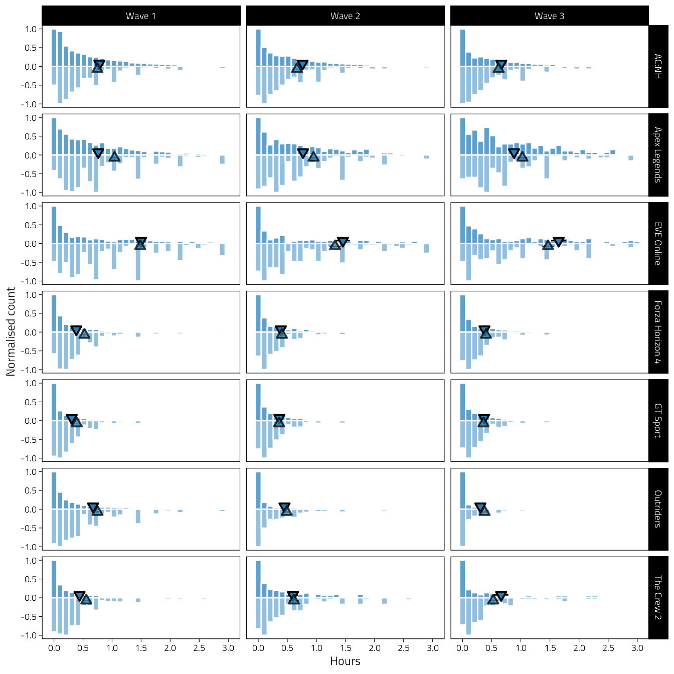

Figure 4.11: Bivariate histograms of average hours played per day by wave (columns) and game (rows). Histograms above zero, with strong colour, reflect behavioural telemetry log data. Histograms below zero, in light colour, indicate subjective estimates of play. Histogram heights are normalized counts. Small triangles indicate means.

A scatterplot of subjective on objective time. Only person-waves with both variables present are included.

d %>%
  drop_na(Hours, hours_est) %>%
  filter(Hours < 3, hours_est < 3) %>%
  select(Game, pid, Wave, Objective = Hours, Subjective = hours_est) %>%
  ggplot(aes(Objective, Subjective)) +
  scale_x_continuous(
    "Hours played per day (behaviour)",
    breaks = c(0, 1, 2, 3), labels = c(0, 1, 2, 3)
  ) +
  scale_y_continuous(
    "Hours played per day (estimate)",
    breaks = pretty_breaks()
  ) +
  geom_point(size = .2, alpha = .2, shape = 1, col = col1) +
  geom_abline(intercept = 0, slope = 1, lty = 2, size = .25) +
  stat_centroid() +
  geom_smooth(
    method = "lm", size = .4,
    color = "black",
    alpha = .33, show.legend = FALSE
  ) +
  facet_grid(Wave ~ Game) +
  theme(aspect.ratio = 1)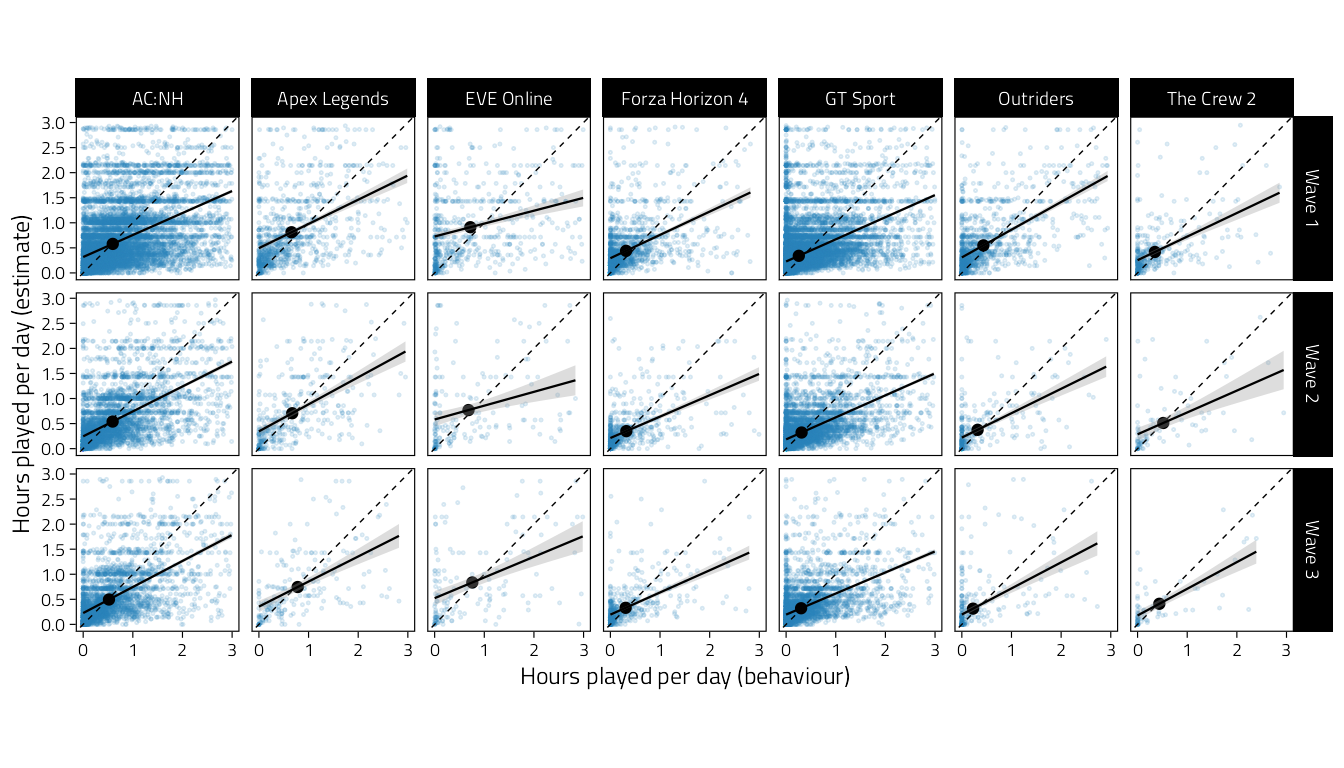

Figure 4.12: Scatterplots of subjectively estimated average hours of daily play on objective behavioural hours played. Dashed line indicates identity, solid lines are simple regression lines. Small blue points are individual participants, and solid dark points are bivariate sample means.

Wave-person differences. Difference indicates estimate - behaviour, so positive numbers indicate overestimates.

d %>%
  select(Game, pid, Wave, Hours, hours_est) %>%
  mutate(Difference = hours_est - Hours) %>%
  filter(Hours < 3, hours_est < 3) %>%
  drop_na(Difference) %>%
  ggplot(aes(Difference, Game)) +
  scale_x_continuous(
    "Estimation error (hours/day)",
    breaks = pretty_breaks()
  ) +
  coord_cartesian(xlim = c(-0.5, 0.5)) +
  geom_vline(xintercept = 0, lty = 2, size = .25) +
  stat_halfeye(point_interval = NULL) +
  stat_summaryh(fun.data = mean_cl_boot_h) +
  facet_wrap("Wave", ncol = 1)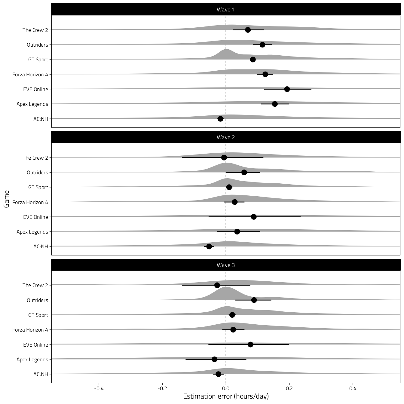

Figure 4.13: Density curves of differences between subjectively estimated and objectively logged average daily play time.

# Overall confidence interval for estimation error
d %>%
  select(Game, pid, Wave, Hours, hours_est) %>%
  mutate(Difference = hours_est - Hours) %>%
  filter(Hours < 3, hours_est < 3) %>%
  drop_na(Difference) %>%
  group_by(Wave) %>%
  summarise(mean_cl_boot(Difference)) %>%
  kbl(digits = 2, caption = "Estimation errors (Estimated - Behaviour)") %>% 
  kable_classic(full_width = FALSE, html_font = Font)

Table 4.7: Estimation errors (Estimated - Behaviour)

Wave	y	ymin	ymax
Wave 1	0.06	0.05	0.06
Wave 2	-0.01	-0.01	0.00
Wave 3	0.01	0.00	0.02

4.5.1 Meta-analysis

fit_ma %>% 
  filter(
    model == "AR",
    Type == "Unstandardized",
    x_var == "Hours",
    y_var %in% c("Affect", "Life satisfaction"),
    Parameter == "wy2 ~ wx1"
  ) %>% 
  select(-posterior) %>% 
  unnest(summary) %>% 
  mutate(
    pd = percent(pd, .1),
    across(where(is.numeric), ~format(round(.x, 2), nsmall = 2)),
    Estimate = str_glue("{Mean} [{CI_low}, {CI_high}]")
  ) %>% 
  select(y_var, Game, Estimate, pd) %>% 
  kbl(caption = "Meta-analytic parameters of subjective time on WB") %>% 
  row_spec(c(8, 16), TRUE) %>% 
  kable_classic(full_width = FALSE, html_font = Font)

Table 4.8: Meta-analytic parameters of subjective time on WB

y_var	Game	Estimate	pd
Affect	AC:NH	0.04 [-0.03, 0.12]	84.5%
Affect	Apex Legends	0.05 [-0.14, 0.28]	68.5%
Affect	EVE Online	0.13 [-0.03, 0.32]	92.9%
Affect	Forza Horizon 4	0.04 [-0.12, 0.23]	68.3%
Affect	GT Sport	-0.04 [-0.12, 0.04]	81.6%
Affect	Outriders	-0.06 [-0.18, 0.04]	86.5%
Affect	The Crew 2	0.03 [-0.19, 0.27]	60.4%
Affect	Average	0.03 [-0.09, 0.16]	67.7%
Life satisfaction	AC:NH	-0.04 [-0.12, 0.05]	82.3%
Life satisfaction	Apex Legends	0.00 [-0.16, 0.29]	62.2%
Life satisfaction	EVE Online	-0.04 [-0.20, 0.15]	74.4%
Life satisfaction	Forza Horizon 4	-0.01 [-0.16, 0.22]	64.8%
Life satisfaction	GT Sport	-0.07 [-0.18, 0.02]	93.9%
Life satisfaction	Outriders	-0.09 [-0.22, 0.01]	95.4%
Life satisfaction	The Crew 2	-0.06 [-0.31, 0.15]	79.9%
Life satisfaction	Average	-0.04 [-0.15, 0.09]	82.4%

4.6 Variability

fit_ma %>% 
  filter(
    model == "AR",
    Type == "Unstandardized",
    y_var %in% c("Affect", "Life satisfaction"),
    x_var == "Hours",
    Parameter == "wy2 ~ wx1"
  ) %>% 
  select(y_var, sd) %>% 
  unnest(sd) %>% 
  kbl(
    caption = "Between game standard deviations of hours -> WB", digits = 2
  ) %>% 
  kable_classic(full_width = FALSE, html_font = Font)

Table 4.9: Between game standard deviations of hours -> WB

y_var	Estimate	Est.Error	Q2.5	Q97.5
Affect	0.11	0.06	0.01	0.27
Life satisfaction	0.08	0.07	0.00	0.26

4.7 System information

sessionInfo()

## R version 4.1.3 (2022-03-10)
## Platform: aarch64-apple-darwin20 (64-bit)
## Running under: macOS Monterey 12.3
## 
## Matrix products: default
## BLAS:   /Library/Frameworks/R.framework/Versions/4.1-arm64/Resources/lib/libRblas.0.dylib
## LAPACK: /Library/Frameworks/R.framework/Versions/4.1-arm64/Resources/lib/libRlapack.dylib
## 
## locale:
## [1] en_US.UTF-8/en_US.UTF-8/en_US.UTF-8/C/en_US.UTF-8/en_US.UTF-8
## 
## attached base packages:
## [1] stats     graphics  grDevices datasets  utils     methods   base     
## 
## other attached packages:
##  [1] broom.mixed_0.2.7 lme4_1.1-27.1     Matrix_1.3-4      cmdstanr_0.4.0   
##  [5] janitor_2.1.0     tidybayes_3.0.1   forcats_0.5.1     stringr_1.4.0    
##  [9] dplyr_1.0.7       purrr_0.3.4       readr_2.0.2       tidyr_1.1.4      
## [13] tibble_3.1.5      tidyverse_1.3.1   multidplyr_0.1.0  lavaan_0.6-9     
## [17] patchwork_1.1.1   cachem_1.0.6      memoise_2.0.1     ggdist_3.0.0     
## [21] ggstance_0.3.5    ggtext_0.1.1      here_1.0.1        ragg_1.1.3       
## [25] brms_2.16.1       Rcpp_1.0.7        bayestestR_0.11.0 ggpp_0.4.2       
## [29] kableExtra_1.3.4  DT_0.19           scales_1.1.1      knitr_1.36       
## [33] ggplot2_3.3.5    
## 
## loaded via a namespace (and not attached):
##   [1] utf8_1.2.2           tidyselect_1.1.1     htmlwidgets_1.5.4   
##   [4] grid_4.1.3           munsell_0.5.0        codetools_0.2-18    
##   [7] miniUI_0.1.1.1       withr_2.4.2          Brobdingnag_1.2-6   
##  [10] colorspace_2.0-2     highr_0.9            rstudioapi_0.13     
##  [13] stats4_4.1.3         bayesplot_1.8.1      emmeans_1.7.2       
##  [16] rstan_2.21.2         mnormt_2.0.2         farver_2.1.0        
##  [19] datawizard_0.2.1     bridgesampling_1.1-2 rprojroot_2.0.2     
##  [22] coda_0.19-4          vctrs_0.3.8          generics_0.1.0      
##  [25] xfun_0.26            R6_2.5.1             markdown_1.1        
##  [28] gamm4_0.2-6          projpred_2.0.2       assertthat_0.2.1    
##  [31] promises_1.2.0.1     nnet_7.3-16          gtable_0.3.0        
##  [34] downlit_0.2.1        processx_3.5.2       rlang_0.4.11        
##  [37] systemfonts_1.0.2    splines_4.1.3        broom_0.7.9         
##  [40] checkmate_2.0.0      inline_0.3.19        yaml_2.2.1          
##  [43] reshape2_1.4.4       abind_1.4-5          modelr_0.1.8        
##  [46] threejs_0.3.3        crosstalk_1.1.1      backports_1.2.1     
##  [49] httpuv_1.6.3         rsconnect_0.8.24     Hmisc_4.6-0         
##  [52] gridtext_0.1.4       tensorA_0.36.2       tools_4.1.3         
##  [55] bookdown_0.24        ellipsis_0.3.2       RColorBrewer_1.1-2  
##  [58] jquerylib_0.1.4      posterior_1.1.0      ggridges_0.5.3      
##  [61] plyr_1.8.6           base64enc_0.1-3      ps_1.6.0            
##  [64] prettyunits_1.1.1    rpart_4.1-15         zoo_1.8-9           
##  [67] cluster_2.1.2        haven_2.4.3          fs_1.5.0            
##  [70] magrittr_2.0.1       data.table_1.14.2    colourpicker_1.1.1  
##  [73] reprex_2.0.1         tmvnsim_1.0-2        mvtnorm_1.1-2       
##  [76] matrixStats_0.61.0   stringfish_0.15.2    qs_0.25.1           
##  [79] hms_1.1.1            shinyjs_2.0.0        mime_0.12           
##  [82] evaluate_0.14        arrayhelpers_1.1-0   xtable_1.8-4        
##  [85] shinystan_2.5.0      jpeg_0.1-9           readxl_1.3.1        
##  [88] gridExtra_2.3        rstantools_2.1.1     compiler_4.1.3      
##  [91] V8_3.4.2             crayon_1.4.1         minqa_1.2.4         
##  [94] StanHeaders_2.21.0-7 htmltools_0.5.2      mgcv_1.8-38         
##  [97] later_1.3.0          tzdb_0.1.2           Formula_1.2-4       
## [100] RcppParallel_5.1.4   RApiSerialize_0.1.0  lubridate_1.8.0     
## [103] DBI_1.1.1            dbplyr_2.1.1         MASS_7.3-54         
## [106] boot_1.3-28          cli_3.0.1            parallel_4.1.3      
## [109] insight_0.14.4       igraph_1.2.6         pkgconfig_2.0.3     
## [112] foreign_0.8-81       xml2_1.3.2           svUnit_1.0.6        
## [115] dygraphs_1.1.1.6     pbivnorm_0.6.0       svglite_2.0.0       
## [118] bslib_0.3.1          webshot_0.5.2        estimability_1.3    
## [121] rvest_1.0.1          snakecase_0.11.0     distributional_0.2.2
## [124] callr_3.7.0          digest_0.6.28        rmarkdown_2.11      
## [127] cellranger_1.1.0     htmlTable_2.2.1      curl_4.3.2          
## [130] shiny_1.7.1          gtools_3.9.2         nloptr_1.2.2.2      
## [133] lifecycle_1.0.1      nlme_3.1-153         jsonlite_1.7.2      
## [136] viridisLite_0.4.0    fansi_0.5.0          pillar_1.6.3        
## [139] lattice_0.20-45      loo_2.4.1            survival_3.2-13     
## [142] fastmap_1.1.0        httr_1.4.2           pkgbuild_1.2.0      
## [145] glue_1.4.2           xts_0.12.1           png_0.1-7           
## [148] shinythemes_1.2.0    stringi_1.7.5        sass_0.4.0          
## [151] textshaping_0.3.5    latticeExtra_0.6-29  renv_0.14.0